Control of an inverted pendulum using PID.
- Inverted Pendulum Control
- Introduction
- Modelling of system
- Control Design and simulation
- Implementation
- Video Demonstration
The inverted pendulum system is unstable, complicated and non-linear. To control the angle of an inverted pendulum efficiently and effectively the PID control strategy is used.
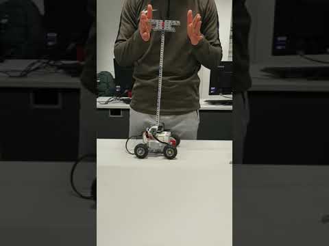
The design shown below is based on the LEGO-Mindstorm EV3, and is a simple cart with two driving wheels, two fixed wheels at the bottom of it, and a pendulum attached to the top part of the cart in order to stabilise the system and help it reach equilibrium. For the pendulum to keep in the upright position, a pendulum head was attached to the top of the rod to try to control it and prevent it from moving back and forth, thus resulting in equilibrium. The total mass of our final design was found to be about 770 grams, including all components added, wires, wheels, etc. The total length of the rod was measured to be about 35.6 cm, however, when getting to the resolving of equations, only half the length of the rod will be used, which is about 17.8 cm. The length of the rod has a direct effect on the motion of the whole design, because the centre of mass changes with the length of the rod, thus resulting in the change of the dynamics of our desired mechanical design.

A focus was placing the pendulum precisely in the middle of the cart in order to focus the centre of mass in the middle of the design to aid in reaching equilibrium. Another focus in our design was on the pendulum length, because as mentioned above, as the length the increases the centre of mass will change accordingly, making it easier for the pendulum to move back and forth. Also the mass of the rod was taken into consideration, as when you decrease the mass, the chance of it staying in equilibrium will be much higher.
The HiTechnic Angle Sensor for the EV3 was used for this project and it determines the displacement of a object in relation to the desired reference position, which in this case is the absolute angle of the pendulum and is placed on its axis of rotation.
To find the two linearised equations of motion for both the cart and the pendulum a description on the modelling of the inverted pendant is shown in the section. The system consists of an inverted rod mounted onto a cart, which can freely move in the X direction as shown in Figure 1.

Figure 1: Pendulum is constrained to move in the vertical plane
L= length of the pendulum
i= inertia of the pendulum
F= force applied to the cart
M= mass of the cart
m= mass of the pendulum
θ= vertical pendulum angle
In order to obtain the dynamics of the system assumptions about how the system perform have been determined. The first assumption is that the system starts at an equilibrium state and that the initial conditions have assumed to be equal to zero. The second assumption is that the pendulum does not move away from the vertical no more than a few degrees in order to satisfy a linear model. The third assumption is that the pendulums brought and the hinge whether pendulums fixed has no friction. The final assumption is that an impulse input is applied to the system in order to displace the pendulum.
For the analysis of the system dynamics equation, Newton’s second law (force= mass * acceleration) was utilised. Figure 1 shows the free body diagram of the system. The distribution of forces of the system is shown in Figure 2. When the pendulum rod inclines with some angle, in the horizontal and vertical directions to force components are resolved.

Figure 2: The forces in the free-body diagram of the cart in the horizontal direction.
P= force exerted by the pendulums in the vertical direction
N= force exerted by the pendant in the horizontal direction
b= friction of the cart
g= force due to gravity
Summing the forces in the vertical direction will grant us no useful information as there is no motion in this direction. Therefore, from the free body diagram, summing the forces of the cart along the horizontal direction, the following equations of motion was deduced that completely define the dynamics of the inverted pendulum:

Equation 1

Equation 2
These two equations, however, are non-linear and need to be linearised in order to carry out our analysis.For the system, the control input will be the force that moves the cart and the outputs will be the carts position and the pendulums angular position. After linearization the two equations of motion obtained the following:

Equation 3

Equation 4
Where u represent the input replacing the force (F).
For our system the following parameters were measured and recorded.
| M | Mass of the cart | 0.7 Kg |
|---|---|---|
| m | Mass of the pendulums | 0.3Kg |
| b | Friction of the cart | 0.1 N/m/sec |
| l | Length of the pendulums | 0.17 m |
| i | Inertia of the pendulums | 0.006Kg.m2 |
| f | For supply to the cart | 1 N |
| g | Force due to gravity | 9.81 m/s2 |
Table 1: Parameters for the inverted pendulum system
For this project the main problem was to control the pendulums position and get it to return to its original vertical position after an initial disturbance (in this case, an impulse force) had been applied therefore, the reference signal was set equal zero. The design requirements for the system are the following:
• Pendulum angle moves no more than 0.1 radians from its original vertical position
• the system has a settling time for the angle of no less than 5 seconds To make the system meet these conditions, different methods of control were used.
PID is very well-known and commonly used feedback controller, due to its reliability and efficiency and consists of three parameters. The proportional gain which acts as a multiplier and multiplies the error response, the integral gain which sums up all the errors produce to reduce the steady-state error and a derivative gain which is the product of the rate of change of the error. It calculates the variation between the measured value and the desired value. And like many controllers It calculates the variation between the measured value and the desired value as shown in Figure 3.

The PID controller was one of the methods used to bring the inverted pendulum equilibrium point when the cart reaches its setpoint.
The PID control equation used to control the pendulum is:

Equation 5
Where u represents the pendant angle control signal and e_θ represents the error angle. The reference angle for the system is set at 0. The system using the PID controller is simulated in MATLAB and SIMULINK.
The purpose of the simulation is to theoretically simulate the outcome of the pendulums. The results from the simulation would then be compared to the practical results to evaluate the difference between the theory and the actual performance of the system.
Simulink was utilised to carry out the simulation for the output responses of the inverted pendulum based on the linearized equations shown in equations 3 and 4. Figure 5 shows the block diagram for the inverted pendulum process (plant) that fully describes our inverted pendulum system based on equations 3 and 4. Here the linearized inverted pendulum modelled, the system parameters used are shown in table 1.

Figure 4:Inverted pendulums process
Figure 5 shows the block diagram of a feedback control loop for the inverted pendulums system with the PID controller. The control system consists of a PID, a plant and a sensor to feedback the output signal. The sensor value is equal to one to simplify the system. The feedback loop begins by having a constant reference signal equalling zero going through the PID controller, which then produces a control signal to act on the actuator, which in this project’s case is a motor voltage signal to give a certain amount of torque to the DC motors to balance the pendulum. The impulses force shown represents the impulse input, the source of disturbance to make the pendulum unbalanced.

Figure 5:PID controller for inverted pendulum
Tuning the PID controller has a large result on the control action of the system and its parameters Kp, Ki and Kd were found through the trial and error method. Using this method, although not optimal, provides satisfactory results and performance for the system.
When tuning our controller, the system was examined on four two cases for Kp values, three for Kd and only once for Ki, as further increase of the integral gain was pointless since the steady-state error approaches zero in an efficiently fast manner.
| Gain | Case 1 | Case 2 | Case 3 | Case 4 |
|---|---|---|---|---|
| Kp | 1 | 120 | 120 | 120 |
| Ki | 1 | 1 | 1 | 1 |
| Kd | 1 | 1 | 10 | 25 |
Case 1: In this case, to see how the system would respond to an impulse disturbance the gains Kp, Ki and Kd are taken as 1. And as shown in figure 8, the system response was unstable as well as the response time was too high. The settling time was also 9.99 seconds which is more 5 seconds desired for the system.

Figure 6: System response for case 1
Case 2: In this case, the Kp value was increased to 120 keeping the values of Ki and Kd unchanged to see how the proportional gain would affect response of the system. The output response was found to be more stable but still some initial oscillations. The settling time of the response was shown to be 0.9654 seconds which is far less than our desired settling time for the system of 5 seconds. However, the peak response reached an amplitude of 0.2277 which is over double the value of our condition of the pendulum not moving then 0.1 rad away from its setpoint.

Figure 7: System response for case 2
Case 3: In this case, the Kd value had increased to 10 to help reduce the overshoot of the system. The output response was found to be quite stable but our system condition of having an amplitude lower than 0.1 has not been met as the peak response for this case is 0.1067.

Figure 8: System response for case 3
Case 4: In the final case, the Kd value was further increased to 25 reducing the overshoot and providing a very stable system that meets all desired control system parameters, giving a peak response of 0.0649 and a settling time of 0.7578 seconds. The simulation of the pendulum does not move more than 0.1 radians away from the desired setpoint, and the time needed for the pendulums to settle to is that setpoint is less than 5 seconds.

Figure 9: System response for case 4
National Instruments LabVIEW is a graphical programming environment suited for high level system design and was the software used to implement our control system design to the actual Lego mind storm inverted pendulum.
Shown in Figure 10, the LabVIEW algorithm begins with an initial countdown lasting five seconds. The time generated from the countdown the pendulums will be put in the desired position which would be closer to the balanced vertical position. Once the countdown finishes the angle sensor will measure what is supposed to be the balanced position of the pendulum and will become the setpoint. The setpoint is going to be the reference value for the pendulum, and the next value that the angle sensor acquires, which would be in the while loop, is going to be compared to the setpoint and the difference between those values will give the error that will be used in the PID controller.
Once the error has been calculated, it enters a case structure, if it is equal to 0 no power will be given to the motors since pendulum would be in a balanced position. If the error is not equal to 0 however, the PID controller shown in Figure 20 will calculate the voltage that will be needed for the motors to balance the pendulum.
Once the summation of the P, I and D controller outputs have been calculated the power of the motor will be obtained. The output value will be put in an ‘In Range and Coerce’ block to limit its values between an upper limit 100 and a lower limit of -100 and tells how fast the motors are going to move in one direction or the other. To determine which direction the motors are going to move in depends on whether the error is less than 0. In the case structure, if the motors are less than 0 they will move forward, if the motors are greater than 0 then it will move backwards. In the true case structure multiplying the PID output value by -1 was to ensure that the motor will go in the opposite direction.

Figure 10:LabVIEW block diagram for the inverted pendulum system
To create the PID control algorithm in LabVIEW, Equation 5 was applied. The error produced from the difference between the setpoint value and the current sensor value was multiplied by the proportional gain (Kp) to obtain the proportional controller output. To create the integral controller output, the past errors of the systems obtained using a shift register, was multiplied by the damping factor variable to help prevent future overshooting of the system. This is then added to the current error of the system, which is then multiplied by the differential in time and the integral gain. The derivative control output was obtained by taking the difference between the actual error of the system and the past error from the previous loop, which was obtained from using another shift register. After the difference in errors is calculated it is then multiplied by the division of the derivative gain and the differential in time. The P, I and D outputs are all then added together to give a PID output control the motors.
Also Both the integral and derivative control outputs are also fed back into a shift register to loop back their respective errors.

Figure 11: PID Control algorithm
Video demonstration of the inverted pendulum system can be seen by clicking the image below: