yulab-smu / aplot Goto Github PK

View Code? Open in Web Editor NEW

92.0 92.0 14.0 2.17 MB

Decorate a plot with associated information

Home Page: https://yulab-smu.top/aplot

Makefile 3.81% R 96.19%

aplot's People

Contributors

Stargazers

Watchers

Forkers

hong-sung-hyun fintrek fionarhuang liangdp1984 darlanminussi xiangpin heroalone king8w imarcello mingli-929 lishensuo gaospecial huerqiang tetukas

aplot's Issues

ordering set with scale__discret(limits = "") switches back to default ggplot2 ordering when using insert_

Hi, thank you so much for providing aplot.

I believe I have found an issue when trying to set a specific order for two different plots.
Here's a reprex to reproduce the issue.

library(aplot)
library(ggplot2)
library(tibble)

set.seed(17)
df <- tibble(id = c("B",
                    "C",
                    "D",
                    "A"),
             sample = c("sp1",
                        "sp2",
                        "sp3",
                        "sp4"),
             value = c(rnorm(1, 1),
                       rnorm(1, 1),
                       rnorm(1, 1),
                       rnorm(1, 1)))

df_anno <- tibble(id = rep("sample", 4),
                  sample = c("sp1",
                             "sp2",
                             "sp3",
                             "sp4"),
                  value = c(rnorm(1, 1),
                            rnorm(1, 1),
                            rnorm(1, 1),
                            rnorm(1, 1)))


p <- ggplot(df) +
  geom_point(aes(x = id,
                 y = sample,
                 size = value)) +
  scale_y_discrete(limits = c("sp3", "sp1", "sp4", "sp2"))

p_anno <- ggplot(df_anno) +
  geom_point(aes(x = id,
                 y = sample,
                 size = value)) +
  scale_y_discrete(limits = c("sp3", "sp1", "sp4", "sp2"))

p %>% 
  insert_left(p_anno)

devtools::session_info()
#> ─ Session info ───────────────────────────────────────────────────────────────
#>  setting  value                       
#>  version  R version 3.6.2 (2019-12-12)
#>  os       Red Hat Enterprise Linux    
#>  system   x86_64, linux-gnu           
#>  ui       unknown                     
#>  language (EN)                        
#>  collate  en_US.UTF-8                 
#>  ctype    en_US.UTF-8                 
#>  tz       America/Chicago             
#>  date     2020-06-26                  
#> 
#> ─ Packages ───────────────────────────────────────────────────────────────────
#>  package     * version date       lib source        
#>  aplot       * 0.0.4   2020-04-07 [1] CRAN (R 3.6.2)
#>  assertthat    0.2.1   2019-03-21 [2] CRAN (R 3.6.0)
#>  backports     1.1.6   2020-04-05 [1] CRAN (R 3.6.2)
#>  callr         3.4.3   2020-03-28 [2] CRAN (R 3.6.2)
#>  cli           2.0.2   2020-02-28 [1] CRAN (R 3.6.2)
#>  colorspace    1.4-1   2019-03-18 [2] CRAN (R 3.6.0)
#>  crayon        1.3.4   2017-09-16 [2] CRAN (R 3.6.0)
#>  desc          1.2.0   2018-05-01 [2] CRAN (R 3.6.0)
#>  devtools      2.3.0   2020-04-10 [1] CRAN (R 3.6.2)
#>  digest        0.6.25  2020-02-23 [2] CRAN (R 3.6.2)
#>  dplyr         0.8.5   2020-03-07 [2] CRAN (R 3.6.2)
#>  ellipsis      0.3.0   2019-09-20 [2] CRAN (R 3.6.0)
#>  evaluate      0.14    2019-05-28 [2] CRAN (R 3.6.0)
#>  fansi         0.4.1   2020-01-08 [1] CRAN (R 3.6.2)
#>  farver        2.0.3   2020-01-16 [1] CRAN (R 3.6.2)
#>  fs            1.4.1   2020-04-04 [1] CRAN (R 3.6.2)
#>  ggplot2     * 3.2.1   2019-08-10 [1] CRAN (R 3.6.2)
#>  glue          1.4.0   2020-04-03 [1] CRAN (R 3.6.2)
#>  gtable        0.3.0   2019-03-25 [2] CRAN (R 3.6.0)
#>  highr         0.8     2019-03-20 [2] CRAN (R 3.6.0)
#>  htmltools     0.4.0   2019-10-04 [2] CRAN (R 3.6.0)
#>  knitr         1.28    2020-02-06 [2] CRAN (R 3.6.2)
#>  labeling      0.3     2014-08-23 [2] CRAN (R 3.6.0)
#>  lazyeval      0.2.2   2019-03-15 [2] CRAN (R 3.6.0)
#>  lifecycle     0.2.0   2020-03-06 [1] CRAN (R 3.6.2)
#>  magrittr      1.5     2014-11-22 [2] CRAN (R 3.6.0)
#>  memoise       1.1.0   2017-04-21 [2] CRAN (R 3.6.0)
#>  munsell       0.5.0   2018-06-12 [2] CRAN (R 3.6.0)
#>  patchwork     1.0.0   2019-12-01 [1] CRAN (R 3.6.2)
#>  pillar        1.4.3   2019-12-20 [2] CRAN (R 3.6.0)
#>  pkgbuild      1.0.6   2019-10-09 [2] CRAN (R 3.6.0)
#>  pkgconfig     2.0.3   2019-09-22 [2] CRAN (R 3.6.0)
#>  pkgload       1.0.2   2018-10-29 [2] CRAN (R 3.6.0)
#>  prettyunits   1.1.1   2020-01-24 [1] CRAN (R 3.6.2)
#>  processx      3.4.2   2020-02-09 [2] CRAN (R 3.6.2)
#>  ps            1.3.2   2020-02-13 [2] CRAN (R 3.6.2)
#>  purrr         0.3.3   2019-10-18 [2] CRAN (R 3.6.0)
#>  R6            2.4.1   2019-11-12 [2] CRAN (R 3.6.0)
#>  Rcpp          1.0.4.6 2020-04-09 [1] CRAN (R 3.6.2)
#>  remotes       2.1.1   2020-02-15 [2] CRAN (R 3.6.2)
#>  rlang         0.4.5   2020-03-01 [1] CRAN (R 3.6.2)
#>  rmarkdown     2.1     2020-01-20 [2] CRAN (R 3.6.2)
#>  rprojroot     1.3-2   2018-01-03 [2] CRAN (R 3.6.0)
#>  scales        1.1.0   2019-11-18 [2] CRAN (R 3.6.0)
#>  sessioninfo   1.1.1   2018-11-05 [2] CRAN (R 3.6.0)
#>  stringi       1.4.6   2020-02-17 [1] CRAN (R 3.6.2)
#>  stringr       1.4.0   2019-02-10 [2] CRAN (R 3.6.0)
#>  testthat      2.3.2   2020-03-02 [2] CRAN (R 3.6.2)
#>  tibble      * 3.0.0   2020-03-30 [2] CRAN (R 3.6.2)
#>  tidyselect    1.0.0   2020-01-27 [2] CRAN (R 3.6.2)
#>  usethis       1.6.0   2020-04-09 [1] CRAN (R 3.6.2)
#>  vctrs         0.2.4   2020-03-10 [2] CRAN (R 3.6.2)
#>  withr         2.1.2   2018-03-15 [2] CRAN (R 3.6.0)
#>  xfun          0.12    2020-01-13 [1] CRAN (R 3.6.2)
#>  yaml          2.2.1   2020-02-01 [2] CRAN (R 3.6.2)

whether need to define operators acting on aplot class?

The insert_right, insert_top etc will return aplot class (eg. p ), which is composed of multiple subplots. They can be extracted using p$plotlist[[1]] etc. And the theme, scale and others of subplot can be adjusted using p$plotlist[[1]] <- p$plotlist[[1]] + xxx. Whether need to define operators acting on this class, then users can use p[[1]] to extract the subplot?

issue when running in jupyter notebook environment

I'm recieving and error when using aplot in a jupyter notebook environment (running R via irkernel).

I install aplot with:

remotes::install_github("YuLab-SMU/aplot")

Example plots:

plt1 <- ggplot(mtcars, aes(x = mpg, y = cyl)) +
  geom_point()
plt2 <- ggplot(mtcars, aes(x = mpg, y = hp)) +
  geom_point()

plt1 %>% aplot::insert_bottom(plt2)

Produces the following error:

ERROR while rich displaying an object: Error in `ggplot_add()`:
! Can't add `x[[i]]` to a ggplot object.

Traceback:
1. tryCatch(withCallingHandlers({
 .     if (!mime %in% names(repr::mime2repr)) 
 .         stop("No repr_* for mimetype ", mime, " in repr::mime2repr")
 .     rpr <- repr::mime2repr[[mime]](obj)
 .     if (is.null(rpr)) 
 .         return(NULL)
 .     prepare_content(is.raw(rpr), rpr)
 . }, error = error_handler), error = outer_handler)
2. tryCatchList(expr, classes, parentenv, handlers)
3. tryCatchOne(expr, names, parentenv, handlers[[1L]])
4. doTryCatch(return(expr), name, parentenv, handler)
5. withCallingHandlers({
 .     if (!mime %in% names(repr::mime2repr)) 
 .         stop("No repr_* for mimetype ", mime, " in repr::mime2repr")
 .     rpr <- repr::mime2repr[[mime]](obj)
 .     if (is.null(rpr)) 
 .         return(NULL)
 .     prepare_content(is.raw(rpr), rpr)
 . }, error = error_handler)
6. repr::mime2repr[[mime]](obj)
7. repr_text.default(obj)
8. paste(capture.output(print(obj)), collapse = "\n")
9. capture.output(print(obj))
10. withVisible(...elt(i))
11. print(obj)
12. print.aplot(obj)
13. grid.draw(x)
14. grid.draw.aplot(x)
15. grid::grid.draw(as.patchwork(x))
16. as.patchwork(x)
17. do.call(plot_list2, y)
18. (function (gglist = NULL, ncol = NULL, nrow = NULL, byrow = NULL, 
  .     widths = NULL, heights = NULL, guides = NULL, labels = NULL, 
  .     tag_levels = NULL, tag_size = 14, design = NULL) 
  . {
  .     p <- Reduce(`+`, gglist, init = plot_filler()) + plot_layout(ncol = ncol, 
  .         nrow = nrow, byrow = byrow, widths = widths, heights = heights, 
  .         guides = guides, design = design)
  .     if (!is.null(tag_levels) || !is.null(labels)) {
  .         pt <- p$theme$plot.tag
  .         if (is.null(pt)) {
  .             pt <- ggplot2::element_text()
  .         }
  .         pt <- modifyList(pt, list(size = tag_size))
  .         p <- p + plot_annotation(tag_levels = tag_levels) & theme(plot.tag = pt)
  .     }
  .     return(p)
  . })(gglist = structure(list(plotlist = list(structure(list(data = structure(list(
  .     mpg = c(21, 21, 22.8, 21.4, 18.7, 18.1, 14.3, 24.4, 22.8, 
  .     19.2, 17.8, 16.4, 17.3, 15.2, 10.4, 10.4, 14.7, 32.4, 30.4, 
  .     33.9, 21.5, 15.5, 15.2, 13.3, 19.2, 27.3, 26, 30.4, 15.8, 
  .     19.7, 15, 21.4), cyl = c(6, 6, 4, 6, 8, 6, 8, 4, 4, 6, 6, 
  .     8, 8, 8, 8, 8, 8, 4, 4, 4, 4, 8, 8, 8, 8, 4, 4, 4, 8, 6, 
  .     8, 4), disp = c(160, 160, 108, 258, 360, 225, 360, 146.7, 
  .     140.8, 167.6, 167.6, 275.8, 275.8, 275.8, 472, 460, 440, 
  .     78.7, 75.7, 71.1, 120.1, 318, 304, 350, 400, 79, 120.3, 95.1, 
  .     351, 145, 301, 121), hp = c(110, 110, 93, 110, 175, 105, 
  .     245, 62, 95, 123, 123, 180, 180, 180, 205, 215, 230, 66, 
  .     52, 65, 97, 150, 150, 245, 175, 66, 91, 113, 264, 175, 335, 
  .     109), drat = c(3.9, 3.9, 3.85, 3.08, 3.15, 2.76, 3.21, 3.69, 
  .     3.92, 3.92, 3.92, 3.07, 3.07, 3.07, 2.93, 3, 3.23, 4.08, 
  .     4.93, 4.22, 3.7, 2.76, 3.15, 3.73, 3.08, 4.08, 4.43, 3.77, 
  .     4.22, 3.62, 3.54, 4.11), wt = c(2.62, 2.875, 2.32, 3.215, 
  .     3.44, 3.46, 3.57, 3.19, 3.15, 3.44, 3.44, 4.07, 3.73, 3.78, 
  .     5.25, 5.424, 5.345, 2.2, 1.615, 1.835, 2.465, 3.52, 3.435, 
  .     3.84, 3.845, 1.935, 2.14, 1.513, 3.17, 2.77, 3.57, 2.78), 
  .     qsec = c(16.46, 17.02, 18.61, 19.44, 17.02, 20.22, 15.84, 
  .     20, 22.9, 18.3, 18.9, 17.4, 17.6, 18, 17.98, 17.82, 17.42, 
  .     19.47, 18.52, 19.9, 20.01, 16.87, 17.3, 15.41, 17.05, 18.9, 
  .     16.7, 16.9, 14.5, 15.5, 14.6, 18.6), vs = c(0, 0, 1, 1, 0, 
  .     1, 0, 1, 1, 1, 1, 0, 0, 0, 0, 0, 0, 1, 1, 1, 1, 0, 0, 0, 
  .     0, 1, 0, 1, 0, 0, 0, 1), am = c(1, 1, 1, 0, 0, 0, 0, 0, 0, 
  .     0, 0, 0, 0, 0, 0, 0, 0, 1, 1, 1, 0, 0, 0, 0, 0, 1, 1, 1, 
  .     1, 1, 1, 1), gear = c(4, 4, 4, 3, 3, 3, 3, 4, 4, 4, 4, 3, 
  .     3, 3, 3, 3, 3, 4, 4, 4, 3, 3, 3, 3, 3, 4, 5, 5, 5, 5, 5, 
  .     4), carb = c(4, 4, 1, 1, 2, 1, 4, 2, 2, 4, 4, 3, 3, 3, 4, 
  .     4, 4, 1, 2, 1, 1, 2, 2, 4, 2, 1, 2, 2, 4, 6, 8, 2)), row.names = c("Mazda RX4", 
  . "Mazda RX4 Wag", "Datsun 710", "Hornet 4 Drive", "Hornet Sportabout", 
  . "Valiant", "Duster 360", "Merc 240D", "Merc 230", "Merc 280", 
  . "Merc 280C", "Merc 450SE", "Merc 450SL", "Merc 450SLC", "Cadillac Fleetwood", 
  . "Lincoln Continental", "Chrysler Imperial", "Fiat 128", "Honda Civic", 
  . "Toyota Corolla", "Toyota Corona", "Dodge Challenger", "AMC Javelin", 
  . "Camaro Z28", "Pontiac Firebird", "Fiat X1-9", "Porsche 914-2", 
  . "Lotus Europa", "Ford Pantera L", "Ferrari Dino", "Maserati Bora", 
  . "Volvo 142E"), class = "data.frame"), layers = list(<environment>), 
  .     scales = <environment>, mapping = structure(list(x = ~mpg, 
  .         y = ~cyl), class = "uneval"), theme = list(), coordinates = <environment>, 
  .     facet = <environment>, plot_env = <environment>, labels = list(
  .         x = "mpg", y = "cyl")), class = c("gg", "ggplot")), structure(list(
  .     data = structure(list(mpg = c(21, 21, 22.8, 21.4, 18.7, 18.1, 
  .     14.3, 24.4, 22.8, 19.2, 17.8, 16.4, 17.3, 15.2, 10.4, 10.4, 
  .     14.7, 32.4, 30.4, 33.9, 21.5, 15.5, 15.2, 13.3, 19.2, 27.3, 
  .     26, 30.4, 15.8, 19.7, 15, 21.4), cyl = c(6, 6, 4, 6, 8, 6, 
  .     8, 4, 4, 6, 6, 8, 8, 8, 8, 8, 8, 4, 4, 4, 4, 8, 8, 8, 8, 
  .     4, 4, 4, 8, 6, 8, 4), disp = c(160, 160, 108, 258, 360, 225, 
  .     360, 146.7, 140.8, 167.6, 167.6, 275.8, 275.8, 275.8, 472, 
  .     460, 440, 78.7, 75.7, 71.1, 120.1, 318, 304, 350, 400, 79, 
  .     120.3, 95.1, 351, 145, 301, 121), hp = c(110, 110, 93, 110, 
  .     175, 105, 245, 62, 95, 123, 123, 180, 180, 180, 205, 215, 
  .     230, 66, 52, 65, 97, 150, 150, 245, 175, 66, 91, 113, 264, 
  .     175, 335, 109), drat = c(3.9, 3.9, 3.85, 3.08, 3.15, 2.76, 
  .     3.21, 3.69, 3.92, 3.92, 3.92, 3.07, 3.07, 3.07, 2.93, 3, 
  .     3.23, 4.08, 4.93, 4.22, 3.7, 2.76, 3.15, 3.73, 3.08, 4.08, 
  .     4.43, 3.77, 4.22, 3.62, 3.54, 4.11), wt = c(2.62, 2.875, 
  .     2.32, 3.215, 3.44, 3.46, 3.57, 3.19, 3.15, 3.44, 3.44, 4.07, 
  .     3.73, 3.78, 5.25, 5.424, 5.345, 2.2, 1.615, 1.835, 2.465, 
  .     3.52, 3.435, 3.84, 3.845, 1.935, 2.14, 1.513, 3.17, 2.77, 
  .     3.57, 2.78), qsec = c(16.46, 17.02, 18.61, 19.44, 17.02, 
  .     20.22, 15.84, 20, 22.9, 18.3, 18.9, 17.4, 17.6, 18, 17.98, 
  .     17.82, 17.42, 19.47, 18.52, 19.9, 20.01, 16.87, 17.3, 15.41, 
  .     17.05, 18.9, 16.7, 16.9, 14.5, 15.5, 14.6, 18.6), vs = c(0, 
  .     0, 1, 1, 0, 1, 0, 1, 1, 1, 1, 0, 0, 0, 0, 0, 0, 1, 1, 1, 
  .     1, 0, 0, 0, 0, 1, 0, 1, 0, 0, 0, 1), am = c(1, 1, 1, 0, 0, 
  .     0, 0, 0, 0, 0, 0, 0, 0, 0, 0, 0, 0, 1, 1, 1, 0, 0, 0, 0, 
  .     0, 1, 1, 1, 1, 1, 1, 1), gear = c(4, 4, 4, 3, 3, 3, 3, 4, 
  .     4, 4, 4, 3, 3, 3, 3, 3, 3, 4, 4, 4, 3, 3, 3, 3, 3, 4, 5, 
  .     5, 5, 5, 5, 4), carb = c(4, 4, 1, 1, 2, 1, 4, 2, 2, 4, 4, 
  .     3, 3, 3, 4, 4, 4, 1, 2, 1, 1, 2, 2, 4, 2, 1, 2, 2, 4, 6, 
  .     8, 2)), row.names = c("Mazda RX4", "Mazda RX4 Wag", "Datsun 710", 
  .     "Hornet 4 Drive", "Hornet Sportabout", "Valiant", "Duster 360", 
  .     "Merc 240D", "Merc 230", "Merc 280", "Merc 280C", "Merc 450SE", 
  .     "Merc 450SL", "Merc 450SLC", "Cadillac Fleetwood", "Lincoln Continental", 
  .     "Chrysler Imperial", "Fiat 128", "Honda Civic", "Toyota Corolla", 
  .     "Toyota Corona", "Dodge Challenger", "AMC Javelin", "Camaro Z28", 
  .     "Pontiac Firebird", "Fiat X1-9", "Porsche 914-2", "Lotus Europa", 
  .     "Ford Pantera L", "Ferrari Dino", "Maserati Bora", "Volvo 142E"
  .     ), class = "data.frame"), layers = list(<environment>), scales = <environment>, 
  .     mapping = structure(list(x = ~mpg, y = ~hp), class = "uneval"), 
  .     theme = list(), coordinates = <environment>, facet = <environment>, 
  .     plot_env = <environment>, labels = list(x = "mpg", y = "hp")), class = c("gg", 
  . "ggplot"))), width = 1, height = c(1, 1), layout = structure(c(1, 
  . 2), .Dim = 2:1), n = 2, main_col = 1, main_row = 1), class = "aplot"))
19. Reduce(`+`, gglist, init = plot_filler())
20. `+.gg`(init, x[[i]])
21. add_ggplot(e1, e2, e2name)
22. ggplot_add(object, p, objectname)
23. ggplot_add.default(object, p, objectname)
24. abort(glue("Can't add `{object_name}` to a ggplot object."))
25. signal_abort(cnd, .file)

However when I run this code in rstudio, I don't encounter any issues.

Have you seen anything like this before? Do you have any ideas how i might fix it?

Coordinate alignment is not perfect.

library(aplot)
library(ggplot2)

set.seed(123)
data1 <- rnorm(1000, mean = -1, sd = 1)
data2 <- rnorm(1000, mean = -2, sd = 2)
data3 <- rnorm(1000, mean = -3, sd = 3)

df1 <- data.frame(
  values = data1,
  group = factor(rep(1, each = 1000))
)

df2 <- data.frame(
  values = data2,
  group = factor(rep(2, each = 1000))
)

df3 <- data.frame(
  values = data3,
  group = factor(rep(3, each = 1000))
)

p1 <- ggplot(df1, aes(x = values, fill = group)) +
  geom_density(alpha = 0.5) +
  labs(title = "P1", x = "value", y = "density", fill = "group") +
  theme_minimal()

p2 <- ggplot(df2, aes(x = values, fill = group)) +
  geom_density(alpha = 0.5) +
  labs(title = "P2", x = "value", y = "density", fill = "group") +
  theme_minimal()

p3 <- ggplot(df3, aes(x = values, fill = group)) +
  geom_density(alpha = 0.5) +
  labs(title = "P3", x = "value", y = "density", fill = "group") +
  theme_minimal()

p1 %>% insert_bottom(p2) %>% insert_bottom(p3)

> sessionInfo()
R version 4.2.1 (2022-06-23)
Platform: aarch64-apple-darwin20 (64-bit)
Running under: macOS Ventura 13.4.1

Matrix products: default
LAPACK: /Library/Frameworks/R.framework/Versions/4.2-arm64/Resources/lib/libRlapack.dylib

locale:
[1] en_US.UTF-8/en_US.UTF-8/en_US.UTF-8/C/en_US.UTF-8/en_US.UTF-8

attached base packages:
[1] stats     graphics  grDevices utils     datasets  methods   base     

other attached packages:
[1] ggplot2_3.4.1 aplot_0.1.10 

loaded via a namespace (and not attached):
 [1] Rcpp_1.0.10          pillar_1.8.1         compiler_4.2.1       cytolib_2.10.0       yulab.utils_0.0.6    tools_4.2.1         
 [7] zlibbioc_1.44.0      lifecycle_1.0.3      tibble_3.2.0         gtable_0.3.1         pkgconfig_2.0.3      rlang_1.1.1         
[13] graph_1.76.0         ggplotify_0.1.0      cli_3.6.1            DBI_1.1.3            rstudioapi_0.14      Rgraphviz_2.42.0    
[19] patchwork_1.1.2      withr_2.5.0          dplyr_1.1.1          gridGraphics_0.5-1   generics_0.1.3       S4Vectors_0.36.1    
[25] vctrs_0.6.3          stats4_4.2.1         grid_4.2.1           tidyselect_1.2.0     glue_1.6.2           data.table_1.14.8   
[31] Biobase_2.58.0       R6_2.5.1             fansi_1.0.4          XML_3.99-0.13        farver_2.1.1         RProtoBufLib_2.10.0 
[37] magrittr_2.0.3       scales_1.2.1         matrixStats_0.63.0   BiocGenerics_0.44.0  flowWorkspace_4.10.1 flowCore_2.10.0     
[43] colorspace_2.1-0     labeling_0.4.2       ncdfFlow_2.44.0      utf8_1.2.3           munsell_0.5.0        ggfun_0.0.9

About plot_list

Hi,

I want to use plot_list to combine pictures, but I found that plot_list will report an error, in fact I can't even run the code of the example, I don't know how to solve it. Below is my code:

library(dplyr)
library(ggplot2)
library(ggstance)
library(ggtree)
library(patchwork)
library(aplot)
no_legend=theme(legend.position='none')

d <- group_by(mtcars, cyl) %>% summarize(mean=mean(disp), sd=sd(disp)) 
d2 <- dplyr::filter(mtcars, cyl != 8) %>% rename(var = cyl)

p1 <- ggplot(d, aes(x=cyl, y=mean)) + 
  geom_col(aes(fill=factor(cyl)), width=1) + 
  no_legend
p2 <- ggplot(d2, aes(var, disp)) + 
  geom_jitter(aes(color=factor(var)), width=.5) + 
  no_legend

p3 <- ggplot(filter(d, cyl != 4), aes(mean, cyl)) + 
  geom_colh(aes(fill=factor(cyl)), width=.6) + 
  coord_flip() + no_legend

pp <- list(p1, p2, p3)
plot_list(pp, ncol=1)

The following is the error:

> plot_list(pp, ncol=1)
Error in UseMethod("as.grob") : 
  no applicable method for 'as.grob' applied to an object of class "list"

The following is the information of the system：

> sessionInfo()
R version 4.1.2 (2021-11-01)
Platform: x86_64-pc-linux-gnu (64-bit)
Running under: Ubuntu 20.04.3 LTS

Matrix products: default
BLAS:   /usr/local/lib/R/lib/libRblas.so
LAPACK: /usr/local/lib/R/lib/libRlapack.so

locale:
 [1] LC_CTYPE=en_US.UTF-8       LC_NUMERIC=C              
 [3] LC_TIME=en_US.UTF-8        LC_COLLATE=en_US.UTF-8    
 [5] LC_MONETARY=en_US.UTF-8    LC_MESSAGES=en_US.UTF-8   
 [7] LC_PAPER=en_US.UTF-8       LC_NAME=C                 
 [9] LC_ADDRESS=C               LC_TELEPHONE=C            
[11] LC_MEASUREMENT=en_US.UTF-8 LC_IDENTIFICATION=C       

attached base packages:
 [1] splines   grid      parallel  stats4    stats     graphics  grDevices
 [8] utils     datasets  methods   base     

other attached packages:
 [1] ggstance_0.3.5.9000                     
 [2] ggtree_3.2.1                            
 [3] aplot_0.1.1                             
 [4] vroom_1.5.7                             
 [5] ggmsa_1.0.0                             
 [6] msaR_0.6.0                              
 [7] ggseqlogo_0.1                           
 [8] patchwork_1.1.1                         
 [9] cowplot_1.1.1                           
[10] tastypie_0.1.0                          
[11] OrgMassSpecR_0.5-3                      
[12] exomePeak2_1.6.1                        
[13] cqn_1.40.0                              
[14] quantreg_5.86                           
[15] SparseM_1.81                            
[16] preprocessCore_1.56.0                   
[17] nor1mix_1.3-0                           
[18] mclust_5.4.8                            
[19] SummarizedExperiment_1.24.0             
[20] MatrixGenerics_1.6.0                    
[21] matrixStats_0.61.0                      
[22] rtracklayer_1.54.0                      
[23] ggsci_2.9                               
[24] tackPlotR_0.0.1                         
[25] MAnorm2_1.2.0                           
[26] cliProfiler_1.0.0                       
[27] circlize_0.4.15                         
[28] ComplexHeatmap_2.10.0                   
[29] TxDb.Hsapiens.UCSC.hg38.knownGene_3.14.0
[30] GenomicFeatures_1.46.1                  
[31] factoextra_1.0.7                        
[32] FactoMineR_2.4                          
[33] ggvenn_0.1.9                            
[34] dplyr_1.0.7                             
[35] customProDB_1.34.0                      
[36] biomaRt_2.50.0                          
[37] AnnotationDbi_1.56.1                    
[38] Biobase_2.54.0                          
[39] impute_1.68.0                           
[40] magrittr_2.0.1                          
[41] antigen.garnish_2.3.0                   
[42] ftrCOOL_2.0.0                           
[43] pROC_1.18.0                             
[44] doParallel_1.0.16                       
[45] iterators_1.0.13                        
[46] foreach_1.5.1                           
[47] caret_6.0-90                            
[48] lattice_0.20-45                         
[49] iq_1.9.3                                
[50] data.table_1.14.2                       
[51] MSstats_4.2.0                           
[52] umap_0.2.7.0                            
[53] limma_3.50.0                            
[54] plotly_4.10.0                           
[55] ggplot2_3.3.5                           
[56] ChIPpeakAnno_3.28.0                     
[57] MetBrewer_0.2.0                         
[58] Cairo_1.5-12.2                          
[59] MSstatsConvert_1.4.1                    
[60] GenomicRanges_1.46.0                    
[61] Biostrings_2.62.0                       
[62] GenomeInfoDb_1.30.0                     
[63] XVector_0.34.0                          
[64] IRanges_2.28.0                          
[65] S4Vectors_0.32.1                        
[66] BiocGenerics_0.40.0                     

loaded via a namespace (and not attached):
  [1] apeglm_1.16.0            ps_1.6.0                 class_7.3-19            
  [4] Rsamtools_2.10.0         rprojroot_2.0.2          crayon_1.4.2            
  [7] rbibutils_2.2.7          MASS_7.3-54              nlme_3.1-153            
 [10] backports_1.3.0          rlang_0.4.12             callr_3.7.0             
 [13] extrafontdb_1.0          nloptr_1.2.2.3           filelock_1.0.2          
 [16] extrafont_0.17           BiocParallel_1.28.0      rjson_0.2.20            
 [19] bit64_4.0.5              glue_1.4.2               processx_3.5.2          
 [22] log4r_0.4.2              regioneR_1.26.0          tidyselect_1.1.1        
 [25] usethis_2.1.3            XML_3.99-0.8             tidyr_1.1.4             
 [28] zoo_1.8-9                proj4_1.0-10.1           GenomicAlignments_1.30.0
 [31] xtable_1.8-4             MatrixModels_0.5-0       Rdpack_2.1.3            
 [34] cli_3.1.0                zlibbioc_1.40.0          rstudioapi_0.13         
 [37] rpart_4.1-15             packcircles_0.3.4        ensembldb_2.18.1        
 [40] lambda.r_1.2.4           treeio_1.18.1            maps_3.4.0              
 [43] askpass_1.1              clue_0.3-60              pkgbuild_1.2.0          
 [46] multtest_2.50.0          cluster_2.1.2            caTools_1.18.2          
 [49] R4RNA_1.22.0             KEGGREST_1.34.0          tibble_3.1.6            
 [52] ggrepel_0.9.1            ape_5.5                  listenv_0.8.0           
 [55] png_0.1-7                permute_0.9-7            future_1.23.0           
 [58] ipred_0.9-12             withr_2.4.2              ggforce_0.3.3           
 [61] bitops_1.0-7             RBGL_1.70.0              plyr_1.8.6              
 [64] AnnotationFilter_1.18.0  coda_0.19-4              pillar_1.6.4            
 [67] gplots_3.1.1             GlobalOptions_0.1.2      cachem_1.0.6            
 [70] fs_1.5.0                 kernlab_0.9-29           scatterplot3d_0.3-41    
 [73] GetoptLong_1.0.5         vctrs_0.3.8              ellipsis_0.3.2          
 [76] generics_0.1.1           devtools_2.4.2           lava_1.6.10             
 [79] tools_4.1.2              tweenr_1.0.2             munsell_0.5.0           
 [82] DelayedArray_0.20.0      pkgload_1.2.3            fastmap_1.1.0           
 [85] compiler_4.1.2           sessioninfo_1.2.1        GenomeInfoDbData_1.2.7  
 [88] prodlim_2019.11.13       InteractionSet_1.22.0    utf8_1.2.2              
 [91] BiocFileCache_2.2.0      recipes_0.1.17           jsonlite_1.7.2          
 [94] scales_1.1.1             graph_1.72.0             tidytree_0.3.6          
 [97] vcfR_1.12.0              genefilter_1.76.0        lazyeval_0.2.2          
[100] reticulate_1.23          checkmate_2.0.0          ash_1.0-15              
[103] statmod_1.4.36           BSgenome_1.62.0          survival_3.2-13         
[106] numDeriv_2016.8-1.1      yaml_2.2.1               ggtranscript_0.99.9     
[109] htmltools_0.5.2          memoise_2.0.0            VariantAnnotation_1.40.0
[112] BiocIO_1.4.0             locfit_1.5-9.4           viridisLite_0.4.0       
[115] digest_0.6.28            assertthat_0.2.1         leaps_3.1               
[118] rappdirs_0.3.3           Rttf2pt1_1.3.9           futile.options_1.0.1    
[121] emdbook_1.3.12           RSQLite_2.2.8            yulab.utils_0.0.4       
[124] future.apply_1.8.1       remotes_2.4.1            VennDiagram_1.7.0       
[127] blob_1.2.2               vegan_2.5-7              futile.logger_1.4.3     
[130] labeling_0.4.2           ProtGenerics_1.26.0      RCurl_1.98-1.5          
[133] hms_1.1.1                colorspace_2.0-2         BiocManager_1.30.16     
[136] shape_1.4.6              nnet_7.3-16              Rcpp_1.0.7              
[139] mvtnorm_1.1-3            ggh4x_0.2.1              fansi_0.5.0             
[142] tzdb_0.2.0               conquer_1.2.1            parallelly_1.28.1       
[145] ModelMetrics_1.2.2.2     R6_2.5.1                 lifecycle_1.0.1         
[148] formatR_1.11             curl_4.3.2               minqa_1.2.4             
[151] testthat_3.1.0           Matrix_1.3-4             desc_1.4.0              
[154] pinfsc50_1.2.0           RColorBrewer_1.1-2       stringr_1.4.0           
[157] gower_0.2.2              htmlwidgets_1.5.4        polyclip_1.10-0         
[160] fmsb_0.7.3               purrr_0.3.4              shadowtext_0.0.9        
[163] gridGraphics_0.5-1       marray_1.72.0            mgcv_1.8-38             
[166] seqmagick_0.1.5          globals_0.14.0           openssl_1.4.5           
[169] flashClust_1.01-2        bdsmatrix_1.3-4          codetools_0.2-18        
[172] lubridate_1.8.0          gtools_3.9.2             prettyunits_1.1.1       
[175] dbplyr_2.1.1             RSpectra_0.16-0          gtable_0.3.0            
[178] DBI_1.1.1                ggfun_0.0.4              httr_1.4.2              
[181] KernSmooth_2.23-20       stringi_1.7.5            progress_1.2.2          
[184] farver_2.1.0             reshape2_1.4.4           uuid_1.0-3              
[187] annotate_1.72.0          timeDate_3043.102        seqinr_4.2-8            
[190] DT_0.19                  xml2_1.3.2               bbmle_1.0.24            
[193] boot_1.3-28              ggalt_0.4.0              lme4_1.1-27.1           
[196] restfulr_0.0.13          ade4_1.7-18              geneplotter_1.72.0      
[199] ggplotify_0.1.0          DESeq2_1.34.0            bit_4.0.4               
[202] pkgconfig_2.0.3          AhoCorasickTrie_0.1.2

How can I fix this problem?

Thanks,
LeeLee

Adding legend

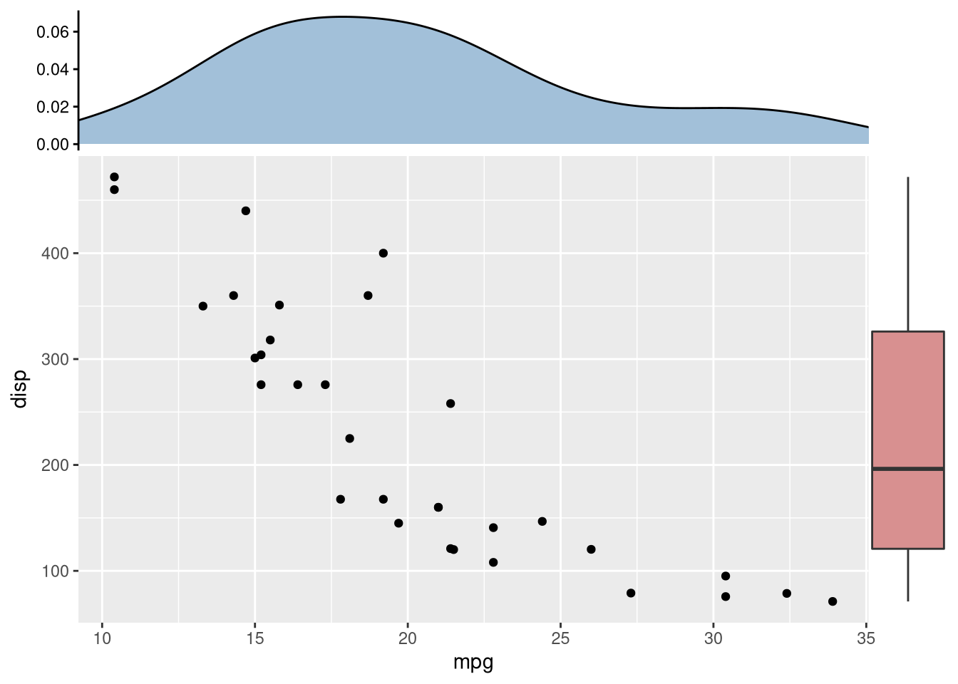
Is that possible to add a legend in the top right corner of this type of plot: https://yulab-smu.top/pkgdocs/pkgdocs_files/figure-html/unnamed-chunk-7-1.png?

Issue with label alignment

Hello,

First off thank you for the wonderful packages ggtree and aplot. They've made plotting my phylogenetic data very easy.

I am running into multiple issues in R using the 'aplot' package, where I am trying to connect a multi-faceted heatmap made with geom_tile in ggplot2, to a tree I have visualized using ggtree. This heatmap includes numeric data for how complete metabolic pathways are for a subset of genomes in my larger phylogenetic tree. Producing this heatmap using gheatmap or appending it to the tree data %<+% hasn't worked because the code for the heatmap is too complex due to the faceting required. Simply trying to insert the tree to the left with common labels returns the error:

Error in xy.coords(x, y, xlabel, ylabel, log) : 'x' is a list, but does not have components 'x' and 'y'

The issues include:

The labels on the y-axis between the tree and heat map are not aligning properly at all despite making sure the syntax and ordering them as a factor are identical
I can only connect the two figures using the following code tree_heatmap<- heatmap %>% insert_left(tree), and I cannot do it the other way around, inserting the heatmap to the right of the tree. When I do so, it says I am supplying discrete values to a continuous scale.
I cannot export the final figure as a PDF, it just shows up blank in the file

Outside of these trials, I can't figure out how to connect these plots working from Figure 7B from this link: https://yulab-smu.top/treedata-book/chapter7.html. I've attached a rough copy and paste image from R studio here to illustrate the alignment issues I am having with the labels.

Really, I am trying to produce the first two panels of Figure 7B, with the proper alignment, label order, and labels dropped for those that are not in the heatmap dataset.

Any help you can provide on this matter would be much appreciated.

Vignette link is broken

Hi! Thanks for the package. It appears that the link to online vignette is broken.

Missing drawing components when combining aplot with geom_fruit

Hi,

I've been struggling to generate a particular composite plot. Nearly all is good except one scale went missing. Hard to explain with text so here are some figures:

Tree figure -

onTip_data <- genus_metadata %>%
  select(c(Diet_specialization, Num_species)) %>%
  rownames_to_column("tip_lable")

g <- ggtree(full_host_genus.tre, right=T, branch.length = 'none') %<+% 
  onTip_data + 
  geom_tippoint(aes(size = Num_species, shape = Diet_specialization)) +
  scale_size(trans="exp", breaks=c(1,2,3)) +
  theme(legend.position = "left")

Then combining with a boxplot using geom_fruit -

g1 <- g + geom_fruit(data=all_metadata, 
                     geom=geom_boxplot,
                     aes(x=Shannon, y=genus),
                     pwidth=1, offset=0.2,
                     grid.params=list(alpha=.5),
                     axis.params=list(axis="x", text=c(0,1,2,3,4,5,6), text.size=2, vjust=1))

Finally combining with a barplot using aplot -

p <- plot_composition(genus_r70k_miAbundFamily.ps, 
                      taxonomic.level="Family", 
                      sample.sort=order_name_list)

p1 <- p + scale_fill_brewer("Microbiota (Family)", palette = "Paired") + 
  guides(fill = guide_legend(ncol = 1)) +
  labs(x="", y="Relative abundance") +
  scale_y_percent() + 
  coord_flip() + 
  theme_ipsum(grid="Y") +
  theme(axis.text.x = element_text(angle=35, hjust=1),
        axis.text.y = element_text(angle=0, hjust=1),
        legend.text = element_text(face = "italic"))

p1 %>% insert_left(g1, width=1)

As you can see that the scale lines from the "Shannon" boxplot are missing and it returned these warnings:

Warning messages:
1: Removed 9 rows containing missing values (geom_segment).
2: Removed 8 rows containing missing values (geom_segment).
3: Removed 7 rows containing missing values (geom_text).

I even try to manually add vertical lines to the final figure but no luck there. Advice please!

Many thanks!
/Ding

online vignette not available

online vignette in README is 404:
https://guangchuangyu.github.io/pkgdocs/aplot.html

Legend position

Hi,
I was wandering if it was possible to adjust legend position.
For instance, in the example from the vignette, i would like to do something like

my.plot = p %>% insert_left(phr, width=.3) %>% 
  insert_right(pp, width=.4)  %>% 
  insert_right(g, width=.4) %>% 
  insert_top(pc, height=.1) %>% 
  insert_top(phc, height=.2)

my.plot + theme(legend.position="bottom")

but i can't make it work...
Thanks this great package and for your help !
Ben

xlim2 fails to align two figures

Hi Y叔,

It seems that xlim2 fail to align two figures that use position

library(tidyr)
library(dplyr)
library(ggplot2)
library(ggtree)
library(aplot)
library(patchwork)

# data to plot heatmap

set.seed(2019-11-07)
d <- matrix(rnorm(25), ncol=5)
rownames(d) <- paste0('g', 1:5)
colnames(d) <- paste0('t', 1:5)
d <- data.frame(d)
d$gene <- rownames(d)
dd <- gather(d, 1:5, key="condition", value='expr')

fig_heat <- ggplot() +
    geom_tile(data = dd, aes(condition, gene, fill=expr),
              position = position_nudge(x = -1)) +
    scale_fill_viridis_c() +
    scale_y_discrete(position="right") +
    theme_minimal() +
    xlab(NULL) + ylab(NULL)

##  points
df_point <- data.frame(condition = paste0("t", 1:5),
                       value = 2:6)
fig_point <- ggplot() +
    geom_point(data = df_point,
               aes(condition, value, size = value,
                   color = condition),
              position = position_nudge(x = -1)) +
    theme_minimal() +
    xlab(NULL) + ylab(NULL)



# align two figures
fig_point + xlim2(fig_heat) + fig_heat + plot_layout(ncol = 1)
fig_heat %>%
    insert_top(fig_point, height = 0.3)

The two figures have the same range

> layer_scales(fig_heat)$x$range
<ggproto object: Class RangeDiscrete, Range, gg>
    range: t1 t2 t3 t4 t5
    reset: function
    train: function
    super:  <ggproto object: Class RangeDiscrete, Range, gg>
> layer_scales(fig_point)$x$range
<ggproto object: Class RangeDiscrete, Range, gg>
    range: t1 t2 t3 t4 t5
    reset: function
    train: function
    super:  <ggproto object: Class RangeDiscrete, Range, gg>

The issue might be due to below, and I am not sure how to overwrite this...

> layer_scales(fig_point)$x$range_c
<ggproto object: Class RangeContinuous, Range, gg>
    range: 0 4
    reset: function
    train: function
    super:  <ggproto object: Class RangeContinuous, Range, gg>
> layer_scales(fig_heat)$x$range_c
<ggproto object: Class RangeContinuous, Range, gg>
    range: -0.5 4.5
    reset: function
    train: function
    super:  <ggproto object: Class RangeContinuous, Range, gg>

Can't save two aplots in one pdf

Hello,

it is not possible to write two aplots on separate pages in one pdf. Only the last plot is shown.

library(ggplot2)
library(ggtree)
library(aplot)

set.seed(2019-10-31)
tr <- rtree(10)

d1 <- data.frame(
  label = c(tr$tip.label[sample(5, 5)], "A"),
  value = sample(1:6, 6))

d2 <- data.frame(
  label = rep(tr$tip.label, 5),
  category = rep(LETTERS[1:5], each=10),
  value = rnorm(50, 0, 3)) 

g <- ggtree(tr) + geom_tiplab(align=TRUE)

p1 <- ggplot(d1, aes(label, value)) + geom_col(aes(fill=label)) + 
  geom_text(aes(label=label, y= value+.1)) +
  coord_flip() + theme_tree2() + theme(legend.position='none')

p2 <- ggplot(d2, aes(x=category, y=label)) + 
  geom_tile(aes(fill=value)) + scale_fill_viridis_c() + 
  theme_tree2() 
p3 <- ggplot(d2, aes(x=category, y=label)) + 
  geom_tile(aes(fill=value)) + 
  theme_tree2()

pdf("test_aplot.pdf", onefile = TRUE)
p2 %>% insert_left(g) %>% insert_right(p1, width=.5) #
p3 %>% insert_left(g) %>% insert_right(p1, width=.5)
dev.off()

Is there a way to resolve that?
Thanks

Can not get right order when connect ggtree and stack barplot in scRNA analysis

Thank you for developmenting the amazing aplot package, yet I have encountered some trouble when using it in scRNA-seq analysis. I intened to connect a ggtree, which is represent the cluster of the samples in data, and a sample-base cell ratio stack barplot. Howerer, no matter how hard I try, I can not get the right order of the samples between these two figure.
Here is my code:

#get cell ratio
Cellratio` <- prop.table(table(sce_sub$CellType, sce_sub$Sample), margin = 2)
Cellratio <- as.data.frame(Cellratio)
colnames(Cellratio) <- c("CellType","id","Abundance")
Cellratio$CellType <- factor(Cellratio$CellType,levels = unique(Cellratio$CellType))
Cellratio <- Cellratio %>% dplyr::select(.,id,Abundance,CellType)

#get tree with ggtree
cellper <- reshape2::dcast(Cellratio,id~CellType, value.var = "Abundance")
rownames(cellper) <- cellper[,1]
cellper <- cellper[,-1]

dis_bray <- vegan::vegdist(cellper, method = 'bray',na.rm = T)
tree <- hclust(dis_bray,method = 'complete')
tree <- ape::as.phylo(tree)

ptest <- ggtree(tree) + 
    geom_tiplab(as_ylab = T)

#get stack bar plot using ggplot2
library(ggthemes)
library(paletteer)
library(aplot)
library(ggstance)

col <- paletteer_d("ggthemes::Classic_20",n=length(unique(meta$CellType)))

p1 <- ggplot(Cellratio) + 
    geom_bar(aes(x = id,
                 y= Abundance,
                 fill = CellType),
             stat = "identity",
             alpha = 0.8) + 
    coord_flip()+
    labs(x='',y = 'Relative Ratio',title ="Cell Abundance")+
    theme(panel.border = element_blank()) + 
    scale_fill_manual(values = col)

p11 <- p1 + 
    scale_y_continuous(expand = c(0,0))+
    theme(
        panel.background = element_rect(fill = NA),
        title = element_text(size = 13,face = "bold"),
        axis.text.x = element_text(size = 12),
        #axis.text.y = element_blank(),
        axis.title = element_text(size = 12,face = "bold"),
        axis.title.y = element_blank())
p11

#using insert_left function to connect these two：
p2 <- p11 %>% aplot::insert_left(.,ptest,width = 1.2)
p2

Yet the order of the samples are not correct....:

I have also tried facet_plot function from ggtree package with no ideal result....
I completely don't know what's wrong and wish to get some help from you.
Thank you very much~

aplot object and ggplot object can't draw in a graph

There is an aplot object which is generated by insert_xxx() and one ggplot object. Now I want to combined the two items, but they can't draw in a graph? what shoud I deal with it?

aplot install error

Hi Yu,

I try to install 'aplot',but I got this error. Could you help me fix it?

install.packages("aplot")
Installing package into ‘/home/xuan/R/x86_64-pc-linux-gnu-library/4.1’
(as ‘lib’ is unspecified)
trying URL 'https://cloud.r-project.org/src/contrib/aplot_0.1.10.tar.gz'
Content type 'application/x-gzip' length 23158 bytes (22 KB)
==================================================
downloaded 22 KB

installing source package ‘aplot’ ...
** package ‘aplot’ successfully unpacked and MD5 sums checked
** using staged installation
** R
** inst
** byte-compile and prepare package for lazy loading
Error: object ‘ggbreak2ggplot’ is not exported by 'namespace:ggfun'
Execution halted
ERROR: lazy loading failed for package ‘aplot’
removing ‘/home/xuan/R/x86_64-pc-linux-gnu-library/4.1/aplot’

The downloaded source packages are in
‘/tmp/RtmpIfk9mI/downloaded_packages’
Warning message:
In install.packages("aplot") :
installation of package ‘aplot’ had non-zero exit status

Problems with the function "insert_left"

When using the aplot package (version 0.2.0), the following error message appears when using the function "insert_left"：

Error in if (zero_range(as.numeric(limits))) { : 
  missing value where TRUE/FALSE needed
In addition: Warning message:
In zero_range(as.numeric(limits)) : NAs introduced by coercion

We have a matrix to plot heatmap like this:

And then we use the following code to generate the cluster tree:

  dd <- dist(plotdata1, method = "euclidean")
  hc <- hclust(dd, method = "ward.D2")
  
  library(ggdendro)
  pa=ggdendrogram(hc,theme_dendro = F)+
    coord_flip()+
    scale_y_reverse()+
    theme_void()

Then the heatmap plot was plotted using the following code:

plotdata1 %>% ggplot(aes(x=condition,y=celltype))+
    geom_tile(aes(fill = value),color = tile_color)+
    scale_y_discrete(expand = c(0,0),position = "right")+
    scale_x_discrete(expand = c(0,0))+
    theme_bw()+
    theme(
      panel.grid = element_blank(),
      axis.title = element_blank(),
      axis.ticks.length = unit(0.15,"cm"),
      axis.text.y.right = element_text(size = 12,colour = "black"),
      axis.text.x.bottom = element_text(size = 12,colour = "black",angle = 0,hjust = 0.5)
    )

And if I want to combine the two plot, Error was occured:

>insert_left(pb,pa,width = relative_width)
Error in if (zero_range(as.numeric(limits))) { : 
  missing value where TRUE/FALSE needed
In addition: Warning message:
In zero_range(as.numeric(limits)) : NAs introduced by coercion

However, aplot (version 0.1.8) works fine whereas vesion 0.1.9 and 0.2.0 can't. So maybe it's necessary to solve this problem in the next vesion.

Alter width of input plot/tree or things to tree, rather than other way around

Hi, firstly wanted to say how much I really love aplot. It has helped me generate a number of great looking figures.

My issue is that I would like to either have my ggtree phylogeny as the input
ggtree_plot %>% insert_right(metadata1, width = 0.5)
but this returns
Error in x$plotlist[[i]] + ylim2(mp) : non-numeric argument to binary operator

So barring that, I would like to be able to scale the input plot
metadata1, width = 0.5 %>% insert_left(g)

Is there any way to do this?

Thanks

zero_range error in 0.1.10

I get the following error in 0.1.10 but everything works fine in 0.1.8 version.
downgrading for now!

library(ggplot2)
library(aplot)

p <- p4 |> insert_left(p1,width = .5)

Error in if (zero_range(as.numeric(limits))) { : 
  missing value where TRUE/FALSE needed
In addition: Warning message:
In zero_range(as.numeric(limits)) : NAs introduced by coercion

labels were covered when applyed insert_left function

Hi，Y叔
I am not good at R programming.
I applyed insert_left function to combine three plots together, but the labels of first plot were covered by the second plot.
I have no idea how to solve this problem, and it will be appreciate if you could give some advice.

How to control the spacing between each plot

Hi,
How to control the spacing between each plot?

Documentation link is broken

In the README, documentation link is provided as:

https://guangchuangyu.github.io/pkgdocs/aplot.html

I clicked it, but got these error messages:

404 Not Found

Sorry, but we couldn't find the page you're looking for.

Adjusting Legend Position with insert_ Functions

Hi,

I am trying to adjust legend position in one of your example. For p2 graph (heatmap like graph). I am interested in to have legend at the bottom of this graph but instead legend for p2 is always coming to the right of the last inserted graph. Is it possible to change guides position after joining graphs ("What I need" on attached picture)?

Thanks,
Dawid

library(ggplot2)
library(ggtree)

set.seed(2019-10-31)
tr <- rtree(10)

d1 <- data.frame(
  # only some labels match
  label = c(tr$tip.label[sample(5, 5)], "A"),
  value = sample(1:6, 6))

d2 <- data.frame(
  label = rep(tr$tip.label, 5),
  category = rep(LETTERS[1:5], each=10),
  value = rnorm(50, 0, 3)) 

# tree
g <- ggtree(tr) + geom_tiplab(align=TRUE)

# p1 = bar_graph
p1 <- ggplot(d1, aes(label, value)) + 
  geom_col(aes(fill=label)) + 
  geom_text(aes(label=label, y= value+.1)) +
  coord_flip() + 
  theme_tree2() + 
  theme(legend.position='none')

# heatmap like graph
p2 <- ggplot(d2, aes(x=category, y=label)) + 
  geom_tile(aes(fill=value)) + scale_fill_viridis_c() +
  theme(legend.position="bottom", legend.box = "horizontal") # adding guide positions

# draw final
p2 %>% insert_left(g) %>% insert_right(p1, width=.5)

[Feature request] Align legend with the start and end of the axis

I wonder if it would be possible to implement a feature that make it possible to align the legend with the start and end of the axis. For example, in the figure below the legend extends along the Y-axis, perfectly aligned with the start and end of the axis. This new feature can be extended to the sharing of a single legend by multiple plots.

(Image taken from https://uk.mathworks.com/help/examples/graphics/win64/CreatingColorbarsFullEmbedExample_01.png)

aplot can not run example.

When I try to run example codes in https://yulab-smu.top/pkgdocs/aplot.html, I got errors.

library(aplot)
no_legend=theme(legend.position='none')
d <- group_by(mtcars, cyl) %>% summarize(mean=mean(disp), sd=sd(disp))
d2 <- dplyr::filter(mtcars, cyl != 8) %>% rename(var = cyl)

p1 <- ggplot(d, aes(x=cyl, y=mean)) +
geom_col(aes(fill=factor(cyl)), width=1) +
no_legend
p2 <- ggplot(d2, aes(var, disp)) +
geom_jitter(aes(color=factor(var)), width=.5) +
no_legend

pp <- list(p1,p2)
plot_list(pp, ncol=1)

output errors:
Error in UseMethod("as.grob") :
no applicable method for 'as.grob' applied to an object of class "list"

r$> sessionInfo()
R version 4.2.3 (2023-03-15)
Platform: x86_64-conda-linux-gnu (64-bit)
Running under: CentOS Linux 7 (Core)

Matrix products: default
BLAS/LAPACK: /cluster/home/shanshenbing/soft/anaconda3/envs/r/lib/libopenblasp-r0.3.21.so

locale:
[1] LC_CTYPE=en_US.UTF-8 LC_NUMERIC=C LC_TIME=en_US.UTF-8 LC_COLLATE=en_US.UTF-8 LC_MONETARY=en_US.UTF-8
[6] LC_MESSAGES=en_US.UTF-8 LC_PAPER=en_US.UTF-8 LC_NAME=C LC_ADDRESS=C LC_TELEPHONE=C
[11] LC_MEASUREMENT=en_US.UTF-8 LC_IDENTIFICATION=C

attached base packages:
[1] stats graphics grDevices utils datasets methods base

other attached packages:
[1] aplot_0.1.10 forcats_1.0.0 stringr_1.5.0 dplyr_1.1.1 purrr_1.0.1 readr_2.1.4 tidyr_1.3.0 tibble_3.2.1
[9] ggplot2_3.4.1 tidyverse_1.3.1

loaded via a namespace (and not attached):
[1] pillar_1.9.0 compiler_4.2.3 cellranger_1.1.0 dbplyr_2.3.2 yulab.utils_0.0.6 tools_4.2.3 jsonlite_1.8.4
[8] lubridate_1.9.2 lifecycle_1.0.3 gtable_0.3.3 timechange_0.2.0 pkgconfig_2.0.3 rlang_1.1.0 reprex_2.0.2
[15] ggplotify_0.1.0 rstudioapi_0.14 DBI_1.1.3 cli_3.6.1 patchwork_1.1.2 haven_2.5.2 xml2_1.3.3
[22] withr_2.5.0 httr_1.4.5 gridGraphics_0.5-1 generics_0.1.3 vctrs_0.6.1 fs_1.6.1 hms_1.1.3
[29] grid_4.2.3 tidyselect_1.2.0 glue_1.6.2 R6_2.5.1 fansi_1.0.4 readxl_1.4.2 farver_2.1.1
[36] tzdb_0.3.0 modelr_0.1.11 magrittr_2.0.3 backports_1.4.1 scales_1.2.1 rvest_1.0.3 colorspace_2.1-0
[43] labeling_0.4.2 utf8_1.2.3 stringi_1.7.12 munsell_0.5.0 broom_1.0.4 ggfun_0.0.9 crayon_1.5.2