zhumengyan / cnmf

Code and example data for running Consensus Non-negative Matrix Factorization on single-cell RNA-Seq data

Consensus Non-negative Matrix factorization (cNMF) v1.2

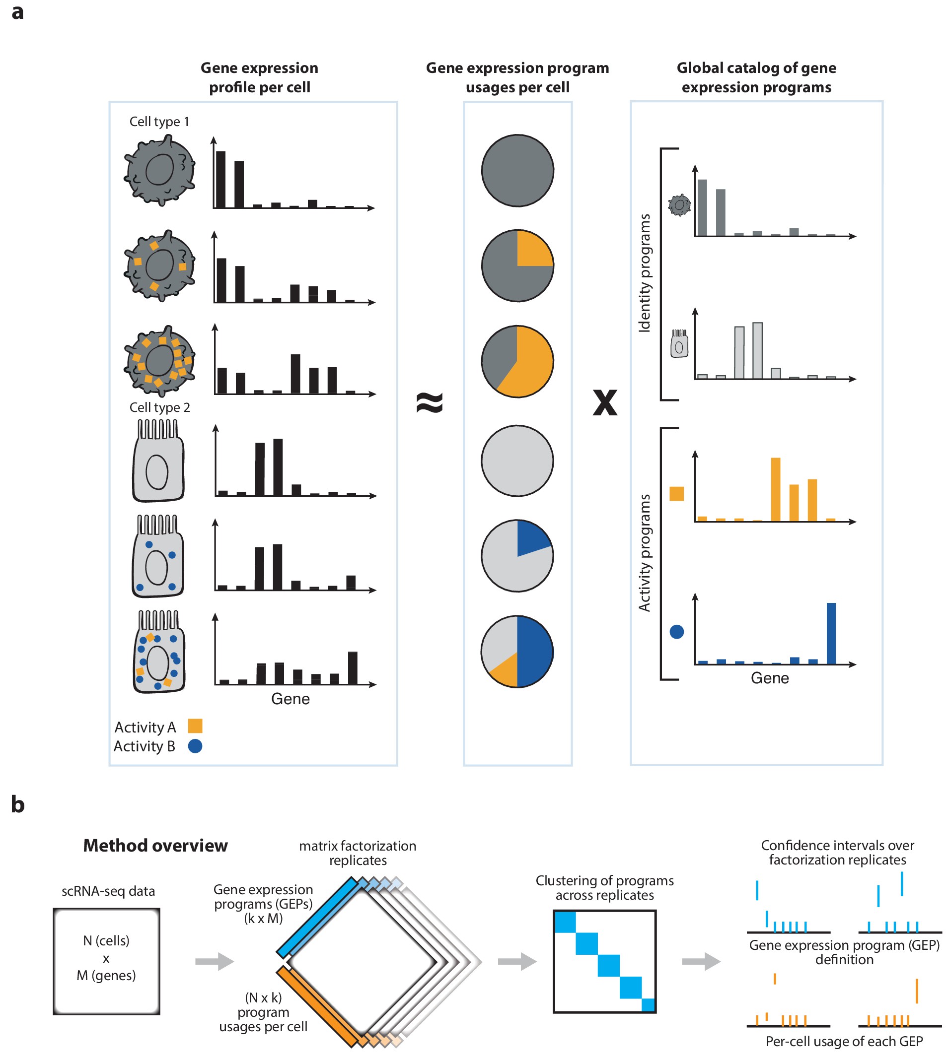
cNMF is an analysis pipeline for inferring gene expression programs from single-cell RNA-Seq (scRNA-Seq) data.

It takes a count matrix (N cells X G genes) as input and produces a (K x G) matrix of gene expression programs (GEPs) and a (N x K) matrix specifying the usage of each program for each cell in the data.

You can read more about the method in the publication here. In addition, the analyses in that paper are available for exploration and re-execution on Code Ocean. You can read more about how to run the cNMF pipeline in this README and can test it out with example data in the included tutorial on simulated data and PBMC tutorial dataset.

Updates from version 1.1

• Increased the threshold for ignoring genes with low mean expression for determining high-variance genes from a TPM of 0.01 to 0.5. Some users were identifying uninterpretable programs with very low usage except in a tiny number of cells. We suspect that this was due to including genes as high-variance that are detected in a small number of cells. This change in the default parameter will help offset that problem in most cases.
• Updated import of NMF for compatibility with scikit-learn versions >22
• Colorbar for heatmaps included with consensus matrix plot

Updates from version 1.0

• Now operates by default on sparse matrices. Use --densify option in prepare step if data is not sparse
• Now takes Scanpy AnnData object files (.h5ad) as input
• Now has option to use KL divergence beta_loss instead of Frobenius. Frobenius is the default because it is much faster.
• Includes a Docker file for creating a Docker container to run cNMF in parallel with cloud compute
• Includes a tutorial on a simple PBMC dataset
• Other minor fixes

Links to previous versions of the code

• cNMF_v1.1.zip
• cNMF_v1.0.zip

Installing cNMF

We provide 2 ways to configure the dependencies for cNMF

Install them using conda

We use conda as a package management system to install the necessary python packages. After installing and configuring conda, you can create an environment for the cNMF workflow using the commands below. These commands install the exact versions of each package that we used for testing and that generated the results in the tutorial notebooks.

# Make sure conda is up to date
conda update -yn base conda
conda create -n cnmf_env --yes --channel bioconda --channel conda-forge --channel defaults python==3.7 fastcluster==1.1.26 matplotlib==3.3.2 numpy==1.19.2 palettable==3.3.0 pandas==1.1.3 scipy==1.5.2 scikit-learn==0.23.2 pyyaml==5.3.1 scanpy==1.6.0 parallel && conda clean --yes --all
conda activate cnmf_env
    
## Only needed to load the example notebook in jupyterlab but not needed for non-interactive runs ## 
conda install --yes jupyterlab==2.2.9 && conda clean --yes --all

Then you need to activate the cnmf_env conda environment each time before running cNMF. With the command below.

conda activate cnmf_env

Run cNMF within a Docker container

We provide a Dockerfile for building a Docker image that is configured for running cNMF.

Alternatively, you can just pull the docker container from quai.io with the command

docker pull quay.io/dkotliar/cnmf:0.2 

Parallelizing the factorization step of cNMF

cNMF runs NMF multiple times and combines the results of each replicates to obtain a more robust consensus estimate. Since many replicates are run, typically for many choices of K, this can be much faster if replicates are run in parallel.

This cNMF code is designed to be agnostic to the method of parallelization. It divides up all of the factorization replicates into a specified number of "workers" which could correspond to cores on a computer, nodes on a compute cluster, or virtual machines in the cloud. In any of these cases, if you are running cNMF for 5 values of K (K= 1..5) and 100 iterations each, there would be 500 total jobs. Those jobs could be divided up amongst 100 workers that would each run 5 jobs, 500 workers that would each run 1 job, or 1 worker that would run all 500 jobs.

You specify the total number of workers in the prepare command (step 1) with the --total-workers flag. Then, for step 2 you run all of the jobs for a specific worker using the --worker-index flag. Step 3 combines the results files that were output by all of the workers. The workers are indexed from 0 to (total-workers - 1).

We provide example commands in the simulated dataset tutorial and the PBMC dataset tutorial for distributing the tasks over multiple cores on a large machine with GNU parallel as well as for distributing them to multiple nodes on an UGER compute cluster. By default, the tutorials do not use any parallelization but simply provide the commands that would be used to run the steps in parallel.

Input data and Scanpy

Input counts data can be provided to cNMF in 2 ways:

1. as a raw tab-delimited text file containing row labels with cell IDs (barcodes) and column labels as gene IDs
2. as a scanpy file ending in .h5ad containg counts as the data feature. See the PBMC dataset tutorial for an example of how to generate the Scanpy object from the data provided by 10X. Because Scanpy uses sparse matrices by default, the .h5ad data structure can take up much less memory than the raw counts matrix and can be much faster to load.

Step by step guide

You can see all possible command line options by running

python cnmf.py --help

and see the simulated dataset tutorial and the PBMC dataset tutorial for a step by step walkthrough with example data. We also describe the key ideas and parameters for each step below.

Step 1 - normalize the input matrix and prepare the run parameters

Example command:

python ./cnmf.py prepare --output-dir ./example_data --name example_cNMF -c ./example_data/counts_prefiltered.txt -k 5 6 7 8 9 10 11 12 13 --n-iter 100 --seed 14 --numgenes 2000

Path structure

• --output-dir - the output directory into which all results will be placed. Default: .
• --name - a subdirectory output_dir/name will be created and all output files will have name as their prefix. Default: cNMF

Input data

• -c - path to the cell x gene counts file. This is expected to be a tab-delimited text file or a Scanpy object saved in the h5ad format
• --tpm [Optional] - Pre-computed Cell x Gene data in transcripts per million or other per-cell normalized data. If none is provided, TPM will be calculated automatically. This can be helpful if a particular normalization is desired. These can be loaded in the same formats as the counts file. Default: None
• --genes-file [Optional] - List of over-dispersed genes to be used for the factorization steps. If not provided, over-dispersed genes will be calculated automatically and the number of genes to use can be set by the --numgenes parameter below. Default: None

Parameters

• -k - space separated list of K values that will be tested for cNMF
• --n-iter - number of NMF iterations to run for each K. Default: 100
• --total-workers - specifies how many workers (e.g. cores on a machine or nodes on a compute farm) can be used in parallel. Default: 1
• --seed - the master seed that will be used to generate the individual seed for each NMF replicate. Default: None
• --numgenes - the number of highest variance genes that will be used for running the factorization. Removing low variance genes helps amplify the signal and is an important factor in correctly inferring programs in the data. However, don't worry, at the end the spectra is re-fit to include estimates for all genes, even those that weren't included in the high-variance set. Default: 2000
• --beta-loss - Loss function for NMF, from one of frobenius, kullback-leibler, itakura-saito. Default: frobenius
• --densify -- Flag indicating that unlike most single-cell RNA-Seq data, the input data is not sparse. Causes the data to be treated as dense. Not recommended for most single-cell RNA-Seq data Default: False

This command generates a filtered and normalized matrix for running the factorizations on. It first subsets the data down to a set of over-dispersed genes that can be provided as an input file or calculated here. While the final spectra will be computed for all of the genes in the input counts file, the factorization is much faster and can find better patterns if it only runs on a set of high-variance genes. A per-cell normalized input file may be provided as well so that the final gene expression programs can be computed with respsect to that normalization.

In addition, this command allocates specific factorization jobs to be run to distinct workers. The number of workers are specified by --total-workers, and the total number of jobs is --n-iter X the number of Ks being tested.

In the example above, we are assuming that no parallelization is to be used (--total-workers 1) and so all of the jobs are being allocated to a single worker.

Please note that the input matrix should not include any cells or genes with 0 total counts. Furthermore if any of the cells end up having 0 counts for the over-dispersed genes, that can cause an error. Please filter out cells and genes with low counts prior to running cNMF.

Step 2 factorize the matrix

Next NMF is run for all of the replicates specified in the previous command. The tasks have been allocated to workers indexed from 0 ... (total-workers -1). You can run all of the NMF replicates allocated to a specific index like below for index 0 corresponding to the first worker:

python ./cnmf.py factorize --output-dir ./example_data --name example_cNMF --worker-index 0 

This is running all of the jobs for worker 1. If you specified a single worker in the prepare step (--total-workers 1) like in the command above, this will run all of the factorizations. However, if you specified more than 1 total worker, you would need to run the commands for those workers as well with separate commands, E.g.:

python ./cnmf.py factorize --output-dir ./example_data --name example_cNMF --worker-index 0 --total-workers 3
python ./cnmf.py factorize --output-dir ./example_data --name example_cNMF --worker-index 1 --total-workers 3
python ./cnmf.py factorize --output-dir ./example_data --name example_cNMF --worker-index 2 --total-workers 3
...

You should submit these commands to distinct processors or machines so they are all run in parallel. See the tutorial on simulated data and PBMC tutorial for examples of how you could submit all of the workers to run in parallel either using GNU parralel or an UGER scheduler.

Tip: The implementation of NMF in scikit-learn by default will use more than 1 core if there are multiple cores on a machine. We find that we get the best performance by using 2 workers when using GNU parallel.

Step 3 combine the individual spectra results files for each K into a merged file

Since a separate file has been created for each replicate for each K, we combine the replicates for each K as below: Example command:

python ./cnmf.py combine --output-dir ./example_data --name example_cNMF

After this, you can optionally delete the individual spectra files like so:

rm ./example_data/example_cNMF/cnmf_tmp/example_cNMF.spectra.k_*.iter_*.df.npz

Step 4 select an optimal K by considering the trade-off between stability and error

This will iterate through all of the values of K that have been run and will calculate the stability and error. It then outputs a PNG image file plotting this relationship into the output_dir/name directory Example command:

python ./cnmf.py k_selection_plot --output-dir ./example_data --name example_cNMF

This outputs a K selection plot to example_data/example_cNMF/example_cNMF.k_selection.png. There is no universally definitive criteria for choosing K but we will typically use the largest value that is reasonably stable and/or a local maximum in stability. See the discussion and methods section and the response to reviewer comments in the manuscript for more discussion about selecting K.

Step 5 obtain consensus estimates for the programs and their usages at the desired value of K

The last step is to cluster the spectra after first optionally filtering out ouliers. This step ultimately outputs 4 files: - GEP estimate in units of TPM - GEP estimate in units of TPM Z-scores, reflecting whether having a higher usage of a program would be expected to decrease or increase gene expression) - Unnormalized GEP usage estimate. - Clustergram diagnostic plot, showing how much consensus there is amongst the replicates and a histogram of distances between each spectra and its K nearest neighbors

We recommend that you use the diagnostic plot to determine the threshold to filter outliers. By default cNMF sets the number of neighbors to use for this filtering as 30% of the number of iterations done. But this can be modified from the command line.

In practice, we tend to run this command twice, once with --local-density-threshold 2.00 to see what the distribution of average distances looks like, and then a second time with --local-density-threshold set to a smaller value determined based on this histogram to filter out outliers. See the tutorials for examples of this.

Example command:

python ./cnmf.py consensus --output-dir ./example_data --name example_cNMF --components 10 --local-density-threshold 0.01 --show-clustering

• --components - value of K to compute consensus clusters for. Must be among the options provided to the prepare step
• --local-density-threshold - the threshold on average distance to K nearest neighbors to use. 2.0 or above means that nothing will be filtered out. Default: 0.5
• --local-neighborhood-size - Percentage of replicates to consider as nearest neighbors for local density filtering. E.g. if you run 100 replicates, and set this to .3, 30 nearest neighbors will be used for outlier detection. Default: 0.3
• --show-clustering - Controls whether or not the clustergram image is output. Default: False

By the end of this step, you should have the following results files in your directory:

• Z-score unit gene expression program matrix - example_data/example_cNMF/example_cNMF.gene_spectra_score.k_10.dt_0_01.txt
• TPM unit gene expression program matrix - example_data/example_cNMF/example_cNMF.gene_spectra_tpm.k_10.dt_0_01.txt
• Usage matrix example_data/example_cNMF/example_cNMF.usages.k_10.dt_0_01.consensus.txt
• Diagnostic plot - example_data/example_cNMF/example_cNMF.clustering.k_10.dt_0_01.pdf

See the tutorials for some subsequent analysis steps that could be used to analyze these results files once they are created.