Introduction
Types of machine learning problems
-
On basis of the nature of the learning “signal” or “feedback” available to a learning system
-
Supervised learning: The computer is presented with example inputs and their desired outputs, given by a “teacher”, and the goal is to learn a general rule that maps inputs to outputs. The training process continues until the model achieves the desired level of accuracy on the training data. Some real-life examples are:
- Image Classification: You train with images/labels. Then in the future, you give a new image expecting that the computer will recognize the new object.
- Market Prediction/Regression: You train the computer with historical market data and ask the computer to predict the new price in the future.
-
Unsupervised learning: No labels are given to the learning algorithm, leaving it on its own to find structure in its input. It is used for the clustering population in different groups. Unsupervised learning can be a goal in itself (discovering hidden patterns in data).
- Clustering: You ask the computer to separate similar data into clusters, this is essential in research and science.
- High Dimension Visualization: Use the computer to help us visualize high dimension data.
- Generative Models: After a model captures the probability distribution of your input data, it will be able to generate more data. This can be very useful to make your classifier more robust.
-
Semi-supervised learning: Problems where you have a large amount of input data and only some of the data is labeled, are called semi-supervised learning problems. These problems sit in between both supervised and unsupervised learning. For example, a photo archive where only some of the images are labeled, (e.g. dog, cat, person) and the majority are unlabeled.
-
Reinforcement learning: A computer program interacts with a dynamic environment in which it must perform a certain goal (such as driving a vehicle or playing a game against an opponent). The program is provided feedback in terms of rewards and punishments as it navigates its problem space.
-
On the basis of “output” desired from a machine-learned system
- Classification: Inputs are divided into two or more classes, outputs are discrete rather than continuous, and the learner must produce a model that assigns unseen inputs to one or more (multi-label classification) of these classes. This is typically tackled in a supervised way. Spam filtering is an example of classification, where the inputs are email (or other) messages and the classes are “spam” and “not spam”.
- Regression: It is also a supervised learning problem, but the outputs are continuous rather than discrete. For example, predicting stock prices using historical data.
- Clustering: Here, a set of inputs is to be divided into groups. Unlike in classification, the groups are not known beforehand, making this typically an unsupervised task.
- Density estimation: The task is to find the distribution of inputs in some space.
- Dimensionality reduction: It simplifies inputs by mapping them into a lower-dimensional space. Topic modeling is a related problem, where a program is given a list of human language documents and is tasked to find out which documents cover similar topics.
Some commonly used machine learning algorithms are Linear Regression, Logistic Regression, Decision Tree, SVM(Support vector machines), Naive Bayes, KNN(K nearest neighbors), K-Means, Random Forest, etc.
https://www.geeksforgeeks.org/getting-started-machine-learning/
Supervised learning
Types of Classifiers (algorithms)
- Linear Classifiers: Logistic Regression
- Tree-Based Classifiers: Decision Tree Classifier
- Support Vector Machines
- Artificial Neural Networks
- Bayesian Regression
- Gaussian Naive Bayes Classifiers
- Stochastic Gradient Descent (SGD) Classifier
- Ensemble Methods: Random Forests, AdaBoost, Bagging Classifier, Voting Classifier, ExtraTrees Classifier
Types of Regression
- Linear regression
- Logistic regression
- Polynomial regression
- Stepwise regression
- Stepwise regression
- Ridge regression
- Lasso regression
- ElasticNet regression
Gradient Descent
Gradient Descent is an optimization algorithm used for minimizing the cost function in various machine learning algorithms. It is basically used for updating the parameters of the learning model.
Types of gradient Descent:
- Batch Gradient Descent: This is a type of gradient descent which processes all the training examples for each iteration of gradient descent. But if the number of training examples is large, then batch gradient descent is computationally very expensive. Hence if the number of training examples is large, then batch gradient descent is not preferred. Instead, we prefer to use stochastic gradient descent or mini-batch gradient descent.
- Stochastic Gradient Descent: This is a type of gradient descent that processes 1 training example per iteration. Hence, the parameters are being updated even after one iteration in which only a single example has been processed. Hence this is quite faster than batch gradient descent. But again, when the number of training examples is large, even then it processes only one example which can be additional overhead for the system as the number of iterations will be quite large.
- Mini Batch gradient descent: This is a type of gradient descent which works faster than both batch gradient descent and stochastic gradient descent. Here b examples where b<m are processed per iteration. So even if the number of training examples is large, it is processed in batches of b training examples in one go. Thus, it works for larger training examples and that too with a lesser number of iterations.
Linear Regression
Linear regression is a statistical approach for modeling the relationship between a dependent variable with a given set of independent variables.
We refer to dependent variables as response and independent variables as features for simplicity.
Simple Linear Regression
Simple linear regression is an approach for predicting a response using a single feature.
Multiple linear regression
Multiple linear regression attempts to model the relationship between two or more features and a response by fitting a linear equation to observed data. Clearly, it is nothing but an extension of Simple linear regression. Consider a dataset with p features(or independent variables) and one response(or dependent variable). Also, the dataset contains n rows/observations.
X (feature matrix) = a matrix of size n X p where x_{ij} denotes the values of jth feature for ith observation.
y (response vector) = a vector of size n where y_{i} denotes the value of response for ith observation.
Polynomial Regression
Advantages of using Polynomial Regression:
- Broad range of function can be fit under it.
- Polynomial basically fits a wide range of curvature.
- Polynomial provides the best approximation of the relationship between the dependent and independent variables.
Disadvantages of using Polynomial Regression
- These are too sensitive to the outliers.
- The presence of one or two outliers in the data can seriously affect the results of nonlinear analysis.
- In addition there are unfortunately fewer model validation tools for the detection of outliers in nonlinear regression than there are for linear regression.
https://www.geeksforgeeks.org/python-implementation-of-polynomial-regression/
Logistic Regression
In a classification problem, the target variable(or output), y, can take only discrete values for a given set of features(or inputs), X.
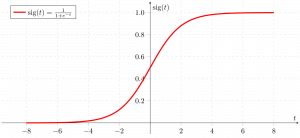
Contrary to popular belief, logistic regression IS a regression model. The model builds a regression model to predict the probability that a given data entry belongs to the category numbered as “1”. Just like Linear regression assumes that the data follows a linear function, Logistic regression models the data using the sigmoid function or *logistic function.


We can infer from the above graph that:
- g(z) tends towards 1 as z -> +infty
- g(z) tends towards 0 as z -> -infty
- g(z) is always bounded between 0 and 1
Logistic regression becomes a classification technique only when a decision threshold is brought into the picture. The setting of the threshold value is a very important aspect of Logistic regression and is dependent on the classification problem itself.
The decision for the value of the threshold value is majorly affected by the values of precision and recall. Ideally, we want both precision and recall to be 1, but this seldom is the case. In case of a Precision-Recall tradeoff we use the following arguments to decide upon the threshold:
-
Low Precision/High Recall: In applications where we want to reduce the number of false negatives without necessarily reducing the number of false positives, we choose a decision value that has a low value of Precision or a high value of Recall. For example, in a cancer diagnosis application, we do not want any affected patient to be classified as not affected without giving much heed to if the patient is being wrongfully diagnosed with cancer. This is because the absence of cancer can be detected by further medical diseases but the presence of the disease cannot be detected in an already rejected candidate.
-
High Precision/Low Recall: In applications where we want to reduce the number of false positives without necessarily reducing the number of false negatives, we choose a decision value that has a high value of Precision or a low value of Recall. For example, if we are classifying customers whether they will react positively or negatively to a personalized advertisement, we want to be absolutely sure that the customer will react positively to the advertisement because otherwise, a negative reaction can cause a loss of potential sales from the customer.
Based on the number of categories, Logistic regression can be classified as:
1. binomial: target variable can have only 2 possible types: “0” or “1” which may represent “win” vs “loss”, “pass” vs “fail”, “dead” vs “alive”, etc.
2. multinomial: target variable can have 3 or more possible types that are not ordered(i.e. types have no quantitative significance) like “disease A” vs “disease B” vs “disease C”.
3. ordinal: it deals with target variables with ordered categories. For example, a test score can be categorized as: “very poor”, “poor”, “good”, “very good”. Here, each category can be given a score like 0, 1, 2, 3.
Confusion Matrix
A much better way to evaluate the performance of a classifier is to look at the confusion matrix. The general idea is to count the number of times instances of class A are classified as class B. Each row in a confusion matrix represents an actual class, while each column represents a predicted class. We want to predict some data using Classification in Machine Learning. Let the classifier be SVM, Decision Tree, Random Forest, Logistic Regression, and so on.
False Positive (type I error)
When we predict that something happens/occurs and it didn't happen/occurred.(rejection of a true null hypothesis) Example: We predict that an earthquake would occur which didn't happen.
False Negative (type II error)
When we predict that something won't happen/occur but it happens/occurs.(non-rejection of a false null hypothesis) Example: We predict that there might be no earthquake but there occurs an earthquake.
Usually, type I errors are considered to be not as critical as type II errors. But in fields like Medicine, Agriculture, both the errors might seem critical.
A 2x2 matrix denoting the right and wrong predictions might help us analyze the rate of success. This matrix is termed the Confusion Matrix.
Representation
The horizontal axis corresponds to the predicted values(y-predicted) and the vertical axis corresponds to the actual values(y-actual).
- [1][1] represents the values that are predicted to be false and are actually false.
- [1][2] represents the values that are predicted to be true but are false.
- [2][1] represents the values that are predicted to be false but are true.
- [2][2] represents the values that are predicted to be true and are actually true.
Using Confusion Matrix in code
Confusion Matrix can be used in python by importing the metrics module from sklearn.
from sklearn import metrics
cm = metrics.confusion_matrix(y_train, y_train_pred)
- Rate of success
r = (TN+TP)/(FN+FP)
from sklearn.metrics import accuracy_score
accuracy_score(y_train, y_train_pred)
- Precision
precision = (TP) / (TP+FP)
TP is the number of true positives, and FP is the number of false positives.
A trivial way to have perfect precision is to make one single positive prediction and ensure it is correct (precision = 1/1 = 100%). This would not be very useful since the classifier would ignore all but one positive instance.
from sklearn.metrics import precision_score
precision_score(y_train, y_train_pred)
- Recall
recall = (TP) / (TP+FN)
from sklearn.metrics import recall_score
recall_score(y_train, y_train_pred)
It is often convenient to combine precision and recall into a single metric called the F1 score, in particular, if you need a simple way to compare two classifiers. The F1 score is the harmonic mean of precision and recall.
# To compute the F1 score, simply call the f1_score() function:
from sklearn.metrics import f1_score
f1_score(y_train, y_train_pred)
The F1 score favors classifiers that have similar precision and recall. This is not always what you want: in some contexts, you mostly care about precision, and in other contexts, you really care about recall. For example, if you trained a classifier to detect videos that are safe for kids, you would probably prefer a classifier that rejects many good videos (low recall) but keeps only safe ones (high precision), rather than a classifier that has a much higher recall but lets a few terrible videos show up in your product (in such cases, you may even want to add a human pipeline to check the classifier’s video selection). On the other hand, suppose you train a classifier to detect shoplifters on surveillance images: it is probably fine if your classifier has only 30% precision as long as it has 99% recall (sure, the security guards will get a few false alerts, but almost all shoplifters will get caught). Unfortunately, you can’t have it both ways: increasing precision reduces recall and vice versa. This is called the precision/recall tradeoff.
https://www.geeksforgeeks.org/confusion-matrix-machine-learning/
https://github.com/Nitin1901/Confusion-Matrix
Binomial Logistic Regression
The likelihood is nothing but the probability of data(training examples), given a model and specific parameter values(here, regression coefficients). It measures the support provided by the data for each possible value of the regression coefficients. And for easier calculations, we take log(likelihood).
The cost function for logistic regression is proportional to the inverse of the likelihood of parameters so that the cost function is minimized using a gradient descent algorithm. where alpha is called learning rate and needs to be set explicitly.
Note: Gradient descent is one of the many ways to estimate regression coefficients.
Basically, these are more advanced algorithms that can be easily run in Python once you have defined your cost function and your gradients. These algorithms are:
- BFGS(Broyden–Fletcher–Goldfarb–Shanno algorithm)
- L-BFGS(Like BFGS but uses limited memory)
- Conjugate Gradient
Advantages/disadvantages of using any one of these algorithms over Gradient descent:
- Advantages
- Don’t need to pick learning rate
- Often run faster (not always the case)
- Can numerically approximate gradient for you (doesn’t always work out well)
- Disadvantages
- More complex
- More of a black box unless you learn the specifics
Multinomial Logistic Regression
In Multinomial Logistic Regression, the output variable can have more than two possible discrete outputs. Consider the Digit Dataset. Here, the output variable is the digit value which can take values out of (0, 12, 3, 4, 5, 6, 7, 8, 9).
At last, here are some points about Logistic regression to ponder upon:
- Does NOT assume a linear relationship between the dependent variable and the independent variables, but it does assume a linear relationship between the logit of the explanatory variables and the response.
- Independent variables can be even the power terms or some other nonlinear transformations of the original independent variables.
- The dependent variable does NOT need to be normally distributed, but it typically assumes a distribution from an exponential family (e.g. binomial, Poisson, multinomial, normal,…); binary logistic regression assumes the binomial distribution of the response.
- The homogeneity of variance does NOT need to be satisfied.
- Errors need to be independent but NOT normally distributed.
- It uses maximum likelihood estimation (MLE) rather than ordinary least squares (OLS) to estimate the parameters and thus relies on large-sample approximations.
Naive Bayes Classifiers
The fundamental Naive Bayes assumption is that each feature makes an:
- independent
- equal
contribution to the outcome.
With relation to our dataset, this concept can be understood as:
- We assume that no pair of features are dependent. For example, the temperature being ‘Hot’ has nothing to do with the humidity or the outlook being ‘Rainy’ has no effect on the winds. Hence, the features are assumed to be independent.
- Secondly, each feature is given the same weight(or importance). For example, knowing the only temperature and humidity alone can’t predict the outcome accurately. None of the attributes is irrelevant and assumed to be contributing equally to the outcome.
Note: The assumptions made by Naive Bayes are not generally correct in real-world situations. In fact, the independence assumption is never correct but often works well in practice.
Other popular Naive Bayes classifiers are:
- Multinomial Naive Bayes: Feature vectors represent the frequencies with which certain events have been generated by a multinomial distribution. This is the event model typically used for document classification.
- Bernoulli Naive Bayes: In the multivariate Bernoulli event model, features are independent booleans (binary variables) describing inputs. Like the multinomial model, this model is popular for document classification tasks, where binary term occurrence(i.e. a word occurs in a document or not) features are used rather than term frequencies(i.e. frequency of a word in the document).
As we reach the end of this article, here are some important points to ponder upon:
- In spite of their apparently over-simplified assumptions, naive Bayes classifiers have worked quite well in many real-world situations, famously document classification and spam filtering. They require a small amount of training data to estimate the necessary parameters.
- Naive Bayes learners and classifiers can be extremely fast compared to more sophisticated methods. The decoupling of the class conditional feature distributions means that each distribution can be independently estimated as a one-dimensional distribution. This in turn helps to alleviate problems stemming from the curse of dimensionality.
https://www.geeksforgeeks.org/naive-bayes-classifiers/
Support Vector Machines(SVMs)
An SVM model is a representation of the examples as points in space, mapped so that the examples of the separate categories are divided by a clear gap that is as wide as possible.
In addition to performing linear classification, SVMs can efficiently perform a non-linear classification, implicitly mapping their inputs into high-dimensional feature spaces.
Decision Tree
- Decision tree algorithm falls under the category of supervised learning. They can be used to solve both regression and classification problems.
- Decision tree uses the tree representation to solve the problem in which each leaf node corresponds to a class label and attributes are represented on the internal node of the tree.
- We can represent any Boolean function on discrete attributes using the decision tree.
Below are some assumptions that we made while using the decision tree:
- In the beginning, we consider the whole training set as the root.
- Feature values are preferred to be categorical. If the values are continuous then they are discretized prior to building the model.
- On the basis of attribute values records are distributed recursively.
- We use statistical methods for ordering attributes as root or the internal node.
- Information Gain
When we use a node in a decision tree to partition the training instances into smaller subsets the entropy changes. Information gain is a measure of this change in entropy.
Entropy
Entropy is the measure of uncertainty of a random variable, it characterizes the impurity of an arbitrary collection of examples. The higher the entropy more the information content.
Building Decision Tree using Information Gain
The essentials:
- Start with all training instances associated with the root node
- Use info gain to choose which attribute to label each node with
- Note: No root-to-leaf path should contain the same discrete attribute twice
- Recursively construct each subtree on the subset of training instances that would be classified down that path in the tree.
The border cases:
- If all positive or all negative training instances remain, a label that node “yes” or “no” accordingly
- If no attributes remain, label with a majority vote of training instances left at that node
- If no instances remain, label with a majority vote of the parent’s training instances
- Gini Index
- Gini Index is a metric to measure how often a randomly chosen element would be incorrectly identified.
- It means an attribute with a lower Gini index should be preferred.
- Sklearn supports the “Gini” criteria for Gini Index and by default, it takes “gini” value.
- The Formula for the calculation of the Gini Index is given below.
The most notable types of decision tree algorithms are:-
- Iterative Dichotomiser 3 (ID3): This algorithm uses Information Gain to decide which attribute is to be used to classify the current subset of the data. For each level of the tree, information gain is calculated for the remaining data recursively.
- C4.5: This algorithm is the successor of the ID3 algorithm. This algorithm uses either Information gain or Gain ratio to decide upon the classifying attribute. It is a direct improvement from the ID3 algorithm as it can handle both continuous and missing attribute values.
- Classification and Regression Tree(CART): It is a dynamic learning algorithm which can produce a regression tree as well as a classification tree depending upon the dependent variable.
Strengths and Weakness of the Decision Tree approach
The strengths of decision tree methods are:
- Decision trees are able to generate understandable rules.
- Decision trees perform classification without requiring much computation.
- Decision trees are able to handle both continuous and categorical variables.
- Decision trees provide a clear indication of which fields are most important for prediction or classification.
The weaknesses of decision tree methods :
- Decision trees are less appropriate for estimation tasks where the goal is to predict the value of a continuous attribute.
- Decision trees are prone to errors in classification problems with many classes and a relatively small numbers of training examples.
- Decision trees can be computationally expensive to train. The process of growing a decision tree is computationally expensive. At each node, each candidate splitting field must be sorted before its best split can be found. In some algorithms, combinations of fields are used and a search must be made for optimal combining weights. Pruning algorithms can also be expensive since many candidate sub-trees must be formed and compared.
https://www.geeksforgeeks.org/decision-tree-introduction-example/
https://www.geeksforgeeks.org/decision-tree/
Random Forest Regression
A Random Forest is an ensemble technique capable of performing both regression and classification tasks with the use of multiple decision trees and a technique called Bootstrap and Aggregation, commonly known as bagging. The basic idea behind this is to combine multiple decision trees in determining the final output rather than relying on individual decision trees.
Random Forest has multiple decision trees as base learning models. We randomly perform row sampling and feature sampling from the dataset forming sample datasets for every model. This part is called Bootstrap.
We need to approach the Random Forest regression technique like any other machine learning technique
- Design a specific question or data and get the source to determine the required data.
- Make sure the data is in an accessible format else convert it to the required format.
- Specify all noticeable anomalies and missing data points that may be required to achieve the required data.
- Create a machine learning model
- Set the baseline model that you want to achieve
- Train the data machine learning model.
- Provide an insight into the model with test data
- Now compare the performance metrics of both the test data and the predicted data from the model.
- If it doesn’t satisfy your expectations, you can try improving your model accordingly or dating your data or use another data modeling technique.
- At this stage you interpret the data you have gained and report accordingly.
Ensemble Classifier
Ensemble learning helps improve machine learning results by combining several models. This approach allows the production of better predictive performance compared to a single model. Basic idea is to learn a set of classifiers (experts) and to allow them to vote.
- Statistical Problem
The Statistical Problem arises when the hypothesis space is too large for the amount of available data. Hence, there are many hypotheses with the same accuracy on the data and the learning algorithm chooses only one of them! There is a risk that the accuracy of the chosen hypothesis is low on unseen data!
- Statistical Problem
The Computational Problem arises when the learning algorithm cannot guarantees finding the best hypothesis.
- Representational Problem
The Representational Problem arises when the hypothesis space does not contain any good approximation of the target class(es).
Main Challenge for Developing Ensemble Models?
The main challenge is not to obtain highly accurate base models, but rather to obtain base models which make different kinds of errors. For example, if ensembles are used for classification, high accuracies can be accomplished if different base models misclassify different training examples, even if the base classifier accuracy is low.
Methods for Independently Constructing Ensembles
- Majority Vote
- Bagging and Random Forest
- Randomness Injection
- Feature-Selection Ensembles
- Error-Correcting Output Coding
Methods for Coordinated Construction of Ensembles
Reliable Classification: Meta-Classifier Approach
Co-Training and Self-Training
Types of Ensemble Classifier
Bagging
Bagging (Bootstrap Aggregation) is used to reduce the variance of a decision tree. Suppose a set D of d tuples, at each iteration i, a training set Di of d tuples is sampled with replacement from D (i.e., bootstrap). Then a classifier model Mi is learned for each training set D < i. Each classifier Mi returns its class prediction. The bagged classifier M* counts the votes and assigns the class with the most votes to X (unknown sample).
Implementation steps of Bagging
- Multiple subsets are created from the original data set with equal tuples, selecting observations with replacement.
- A base model is created on each of these subsets.
- Each model is learned in parallel from each training set and independent of each other.
- The final predictions are determined by combining the predictions from all the models.
Random Forest
Random Forest is an extension over bagging. Each classifier in the ensemble is a decision tree classifier and is generated using a random selection of attributes at each node to determine the split. During classification, each tree votes, and the most popular class is returned.
Implementation steps of Random Forest
- Multiple subsets are created from the original data set, selecting observations with replacement.
- A subset of features is selected randomly and whichever feature gives the best split is used to split the node iteratively.
- The tree is grown to the largest.
- Repeat the above steps and prediction is given based on the aggregation of predictions from n number of trees.
Voting Classifier
A Voting Classifier is a machine learning model that trains on an ensemble of numerous models and predicts an output (class) based on their highest probability of chosen class as the output.
It simply aggregates the findings of each classifier passed into Voting Classifier and predicts the output class based on the highest majority of voting. The idea is instead of creating separate dedicated models and finding the accuracy for each of them, we create a single model that trains by these models and predicts output based on their combined majority of voting for each output class.
Voting Classifier supports two types of votings.
- Hard Voting: In hard voting, the predicted output class is a class with the highest majority of votes i.e the class which had the highest probability of being predicted by each of the classifiers. Suppose three classifiers predicted the output class(A, A, B), so here the majority predicted A as output. Hence A will be the final prediction.
- Soft Voting: In soft voting, the output class is the prediction based on the average of probability given to that class. Suppose given some input to three models, the prediction probability for class A = (0.30, 0.47, 0.53) and B = (0.20, 0.32, 0.40). So the average for class A is 0.4333 and B is 0.3067, the winner is clearly class A because it had the highest probability averaged by each classifier.
Unsupervised learning