![]()
All about orthogonal polynomials.


orthopy provides various orthogonal polynomial classes for lines, triangles, disks, spheres, n-cubes, the nD space with weight function exp(-r2) and more. All computations are done using numerically stable recurrence schemes. Furthermore, all functions are fully vectorized and can return results in exact arithmetic.
Install orthopy from PyPI with
pip install orthopy
Licenses for personal and academic use can be purchased here. You'll receive a confirmation email with a license key. Install the key with
plm add <your-license-key>
on your machine and you're good to go.
For commercial use, please contact [email protected].
The main function of all submodules is the iterator Eval which evaluates the series of
orthogonal polynomials with increasing degree at given points using a recurrence
relation, e.g.,
import orthopy

x = 0.5

evaluator = orthopy.c1.legendre.Eval(x, "classical")
for _ in range(5):
     print(next(evaluator))
1.0 # P_0(0.5)
0.5 # P_1(0.5)
-0.125 # P_2(0.5)
-0.4375 # P_3(0.5)
-0.2890625 # P_4(0.5)Other ways of getting the first n items are
evaluator = Eval(x, "normal")
vals = [next(evaluator) for _ in range(n)]

import itertools
vals = list(itertools.islice(Eval(x, "normal"), n))
Instead of evaluating at only one point, you can provide any array for x; the
polynomials will then be evaluated for all points at once. You can also use sympy for
symbolic computation:
import itertools
import orthopy
import sympy

x = sympy.Symbol("x")

evaluator = orthopy.c1.legendre.Eval(x, "classical")
for val in itertools.islice(evaluator, 5):
     print(sympy.expand(val))
1
x
3*x**2/2 - 1/2
5*x**3/2 - 3*x/2
35*x**4/8 - 15*x**2/4 + 3/8
All Eval methods have a scaling argument which can have three values:
"monic": The leading coefficient is 1."classical": The maximum value is 1 (or (n+alpha over n))."normal": The integral of the squared function over the domain is 1.
For univariate ("one-dimensional") integrals, every new iteration contains one function. For bivariate ("two-dimensional") domains, every level will contain one function more than the previous, and similarly for multivariate families. See the tree plots below.
 |
 |
 |
|---|---|---|
| Legendre | Chebyshev 1 | Chebyshev 2 |
Jacobi, Gegenbauer (α=β), Chebyshev 1 (α=β=-1/2), Chebyshev 2 (α=β=1/2), Legendre (α=β=0) polynomials.
import orthopy

orthopy.c1.legendre.Eval(x, "normal")
orthopy.c1.chebyshev1.Eval(x, "normal")
orthopy.c1.chebyshev2.Eval(x, "normal")
orthopy.c1.gegenbauer.Eval(x, "normal", lmbda)
orthopy.c1.jacobi.Eval(x, "normal", alpha, beta)
The plots above are generated with
import orthopy

orthopy.c1.jacobi.show(5, "normal", 0.0, 0.0)
# plot, savefig also exist
Recurrence coefficients can be explicitly retrieved by
import orthopy

rc = orthopy.c1.jacobi.RecurrenceCoefficients(
    "monic",  # or "classical", "normal"
    alpha=0, beta=0, symbolic=True
)
print(rc.p0)
for k in range(5):
    print(rc[k])
1
(1, 0, None)
(1, 0, 1/3)
(1, 0, 4/15)
(1, 0, 9/35)
(1, 0, 16/63)

(Generalized) Laguerre polynomials.
evaluator = orthopy.e1r.Eval(x, alpha=0, scaling="normal")
Hermite polynomials come in two standardizations:
"physicists"(against the weight functionexp(-x ** 2)"probabilists"(against the weight function1 / sqrt(2 * pi) * exp(-x ** 2 / 2)
evaluator = orthopy.e1r2.Eval(
    x,
    "probabilists",  # or "physicists"
    "normal"
)
Not all of those are polynomials, so they should really be called associated Legendre functions. The kth iteration contains 2k+1 functions, indexed from -k to k. (See the color grouping in the above plot.)
evaluator = orthopy.c1.associated_legendre.Eval(
    x, phi=None, standardization="natural", with_condon_shortley_phase=True
)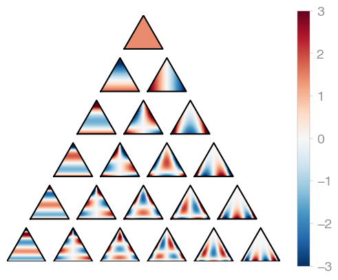
orthopy's triangle orthogonal polynomials are evaluated in terms of barycentric
coordinates, so the
X.shape[0] has to be 3.
import orthopy

bary = [0.1, 0.7, 0.2]
evaluator = orthopy.t2.Eval(bary, "normal")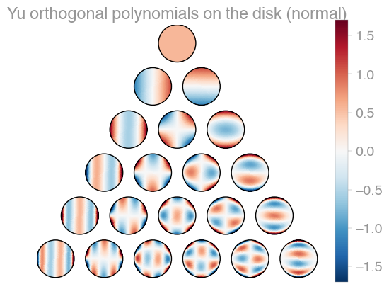 |
 |
 |
|---|---|---|
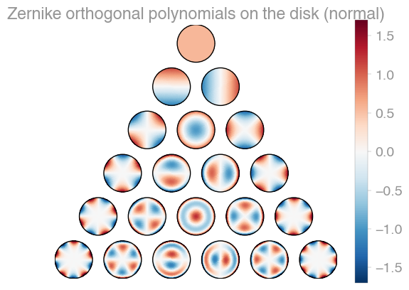
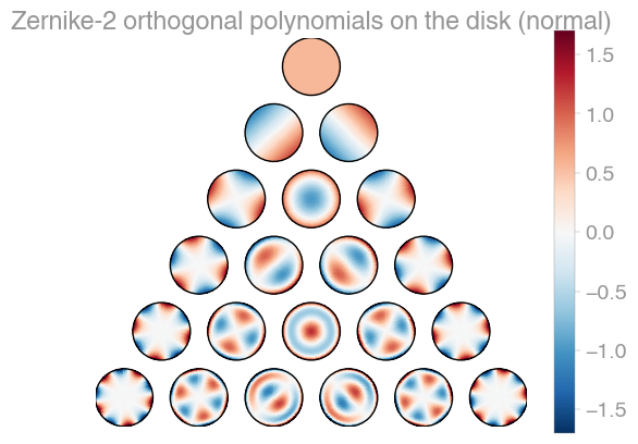
| Xu | Zernike | Zernike 2 |
orthopy contains several families of orthogonal polynomials on the unit disk: After Xu, Zernike, and a simplified version of Zernike polynomials.
import orthopy

x = [0.1, -0.3]

evaluator = orthopy.s2.xu.Eval(x, "normal")
# evaluator = orthopy.s2.zernike.Eval(x, "normal")
# evaluator = orthopy.s2.zernike2.Eval(x, "normal")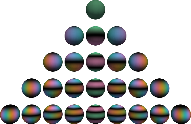
Complex-valued spherical harmonics, (black=zero, green=real positive, pink=real negative, blue=imaginary positive, yellow=imaginary negative). The functions in the middle are real-valued. The complex angle takes n turns on the nth level.
evaluator = orthopy.u3.EvalCartesian(
    x,
    scaling="quantum mechanic"  # or "acoustic", "geodetic", "schmidt"
)

evaluator = orthopy.u3.EvalSpherical(
    theta_phi,  # polar, azimuthal angles
    scaling="quantum mechanic"  # or "acoustic", "geodetic", "schmidt"
) |
 |
 |
|---|---|---|
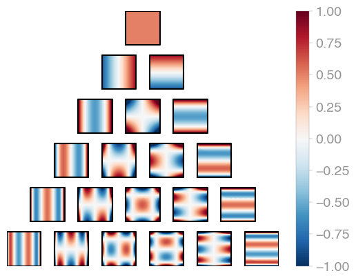
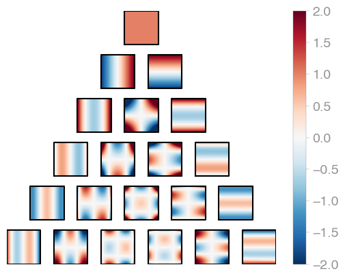
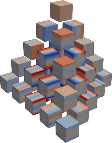
| C1 (Legendre) | C2 | C3 |
Jacobi product polynomials.
All polynomials are normalized on the n-dimensional cube. The dimensionality is
determined by X.shape[0].
evaluator = orthopy.cn.Eval(X, alpha=0, beta=0)
values, degrees = next(evaluator) |
 |
 |
|---|---|---|
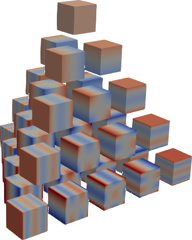
| E1r2 | E2r2 | E3r2 |
Hermite product polynomials.
All polynomials are normalized over the measure. The dimensionality is determined by
X.shape[0].
evaluator = orthopy.enr2.Eval(
    x,
    standardization="probabilists"  # or "physicists"
)
values, degrees = next(evaluator)-
Generating recurrence coefficients for 1D domains with Stieltjes, Golub-Welsch, Chebyshev, and modified Chebyshev.
-
The the sanity of recurrence coefficients with test 3 from Gautschi's article: computing the weighted sum of orthogonal polynomials:
orthopy.tools.gautschi_test_3(moments, alpha, beta)
-
Clenshaw algorithm for computing the weighted sum of orthogonal polynomials:
vals = orthopy.c1.clenshaw(a, alpha, beta, t)
- Robert C. Kirby, Singularity-free evaluation of collapsed-coordinate orthogonal polynomials, ACM Transactions on Mathematical Software (TOMS), Volume 37, Issue 1, January 2010
- Abedallah Rababah, Recurrence Relations for Orthogonal Polynomials on Triangular Domains, MDPI Mathematics 2016, 4(2)
- Yuan Xu, Orthogonal polynomials of several variables, arxiv.org, January 2017