ncss-tech / soildb

soilDB: Simplified Access to National Cooperative Soil Survey Databases

Installation

Get the stable version from CRAN:

install.packages('soilDB', dependencies = TRUE)

Get the development version from GitHub:

remotes::install_github("ncss-tech/soilDB", dependencies = FALSE)

Website

• CRAN Package: https://cran.r-project.org/package=soilDB
• Package Manual: http://ncss-tech.github.io/soilDB/
• Algorithms for Quantitative Pedology (AQP) Project: http://ncss-tech.github.io/AQP/

Citation

## To cite soilDB in publications use:
## 
##   Beaudette, D., Skovlin, J., Roecker, S., Brown, A. (2024). soilDB:
##   Soil Database Interface. R package version 2.8.2.
##   <https://CRAN.R-project.org/package=soilDB>
## 
## A BibTeX entry for LaTeX users is
## 
##   @Manual{,
##     title = {soilDB: Soil Database Interface},
##     author = {Dylan Beaudette and Jay Skovlin and Stephen Roecker and Andrew Brown},
##     note = {R package version 2.8.2},
##     url = {https://CRAN.R-project.org/package=soilDB},
##     year = {2024},
##   }

soilDB 2.8.3

Functions by Data Source

• Soil Data Access (SDA)
  • fetchSDA
  • fetchSDA_spatial
  • SDA_query
  • SDA_spatialQuery
  • “SSURGO On Demand” Queries
    • get_SDA_hydric
    • get_SDA_interpretation
    • get_SDA_muaggatt
    • get_SDA_pmgroupname
    • get_SDA_property
    • get_SDA_coecoclass
    • get_SDA_metrics
    • get_SDA_cosurfmorph
• SSURGO Web Soil Survey
  • downloadSSURGO
  • createSSURGO
• SSURGO Local Geodatabases
  • fetchGDB
• ROSETTA
  • ROSETTA
• SSURGO/KSSL via SoilWeb
  • fetchKSSL
  • fetchOSD
  • siblings
  • OSDquery
  • seriesExtent
  • taxaExtent
  • mukey.wcs
  • ISSR800.wcs
• NASIS WWW interface
  • parseWebReport
  • fetchNASISWebReport
• SCAN/SNOTEL
  • fetchSCAN
  • SCAN_SNOTEL_metadata
• Henry Mount Soil and Water Database
  • fetchHenry
• NASIS local database
  • fetchNASIS
  • dbConnectNASIS (alias NASIS())
  • dbQueryNASIS
  • createStaticNASIS
• SoilGrids
  • fetchSoilGrids

Miscellaneous Functions

• estimateSTR
• STRplot
• KSSL_VG_model
• simplifyFragmentData
• simplifyColorData
• uncode
• code
• get_NOAA_GHCND

Tutorials and Demonstrations

• fetchKSSL
• SDA_query
• fetchOSD
• SCAN/SNOTEL Data

Related Packages

• aqp
• sharpshootR
• SoilTaxonomy

soildb's Issues

volume % fragments, excluding parafrags

On branch 'Parafractions' (commit 6e576a4) simplifyFragmentData() outputs a dataframe with an additional column total_frags_pct_nopf. This is calculated in the same way as total_frags_pct except it omits the columns containing the "para"-fractions from the row sum calculation on the phfrags-derived dataframe.

Therefore, functions relying on fetchNASIS() or other functions that use simplifyFragmentData() will now have another variable available reflecting the parafragment-free totals.

get_phlabresults_data_from_NASIS_db()

need fix for when sample depths are empty

INNER or LEFT joins for component parent material and geomorph data

Functions affected:

• get_component_cogeomorph_data_from_NASIS_db() -- commit 8cb1201
• get_component_copm_data_from_NASIS_db() -- commit 94aa357

INNER JOINS implicitly filter NULL records, LEFT JOINS retain them.

For example, before is based on the LEFT JOIN, after is based on the INNER JOIN:

un-mixing SSURGO / STATSGO in SDA

get_component_from_SDA(WHERE = "compname = 'Miami'") is returning duplicates even though the duplicates argument is set to FALSE. Apparently it's also pulling STATSGO mapunit types. Need to include mapunit type in get or remove and write separate get for STASTGO.

NASIS geomorphic feature query has joins without join constraint

Review this:

SELECT pedon_View_1.peiid, sitegeomordesc_View_1.geomfmod, geomorfeat.geomfname, sitegeomordesc_View_1.geomfeatid, sitegeomordesc_View_1.existsonfeat, sitegeomordesc_View_1.geomfiidref, lower(geomorfeattype.geomftname) as geomftname
  
  FROM geomorfeattype 
  RIGHT JOIN geomorfeat 
  RIGHT JOIN site_View_1 INNER JOIN sitegeomordesc_View_1 ON site_View_1.siteiid = sitegeomordesc_View_1.siteiidref
  INNER JOIN siteobs_View_1 INNER JOIN pedon_View_1 ON siteobs_View_1.siteobsiid = pedon_View_1.siteobsiidref
  ON site_View_1.siteiid = siteobs_View_1.siteiidref
  ON geomorfeat.geomfiid = sitegeomordesc_View_1.geomfiidref
  ON geomorfeattype.geomftiid = geomorfeat.geomftiidref 
  ORDER BY peiid, geomfeatid ASC;

fetchNASIS and fetchNASIS_component_data need proper manual pages

soil texture plotting / subsetting / flagging helper function or guidance

multiple sensors -- fetchSCAN

There are some SCAN/SNOTEL stations with multiple (above-ground) sensors per sensor prefix. For example:

library(soilDB)
m <- SCAN_sensor_metadata(site.code=c(482,613))
m[, 1:3]

   site.code      Label                    Element
1        482   WTEQ.I-1      Snow Water Equivalent
2        482   WTEQ.I-2      Snow Water Equivalent
3        482   PREC.I-1 Precipitation Accumulation
4        482   PREC.I-2 Precipitation Accumulation
5        482   TOBS.I-1   Air Temperature Observed
6        482   TOBS.I-2   Air Temperature Observed
7        482   TOBS.I-3   Air Temperature Observed
8        482   TMAX.D-1    Air Temperature Maximum
9        482   TMIN.D-1    Air Temperature Minimum

As of ab70a98 fetchSCAN() will issue a message and then naively use the first sensor.

A better solution would require significant changes to fetchSCAN() and / or working with SCAN admins.

update all NASIS queries that involve domains to use uncode()

This is mostly done as of c9839ec (thanks Jay).

There are still some references to metadata_domain_detail:

• 1 get_colors_from_pedon_db.R
• 19 get_extended_data_from_pedon_db.R
• 3 get_hz_data_from_pedon_db.R
• 12 get_site_data_from_pedon_db.R

New functions for horizon subsetting and selection within an SPC

There are times when it would be nice to subset horizons within and SPC, without having to manually extract / subset / replace data.

Current approach, not ideal:

h <- horizons(spc)
# do something to h
horizons(spc) <- h

Better approach:

spc <- subsetHorizons(spc, expression, ...)

Building on subsetHorizons(), the selectHorizonsByDepth(spc, z=c(5, 15)) function would return a SoilProfileCollection including only those horizons that intersect depths of 5 and 15 cm.

Thinking this through some more, an ever better approach would use the [] notation for extraction of horizon data, possibly with new operators. Like this:

# return an SPC with just those horizons that *intersect* the depth interval of 5-10m.
x <- spc[, %intersect% c(5,10)]

SDA example must explicitly filter out STATSGO records

See (#25) for context.

All queries in the manual pages and tutorials need this:

-- critical: filter out STATSGO data
AND legend.areasymbol != 'US'

add testing suite

http://r-pkgs.had.co.nz/tests.html

document `KSSL_VG_model()`

This is a new function in soilDB that can utilize the recently added (2016-11-17) Rosetta / VG parameters now returned by fetchKSSL().

add some queries to accommodate the new ncss_pedon_lab_data tables

simplfyFragmentData() needs a full review

This is after switching to uncode() in fetchNASIS_pedons().

SDA and duplicate records

Trying to get my head around this one.

An example from Stephen:

library(soilDB)
library(daff)

# test both cases, thanks Stephen for the example
x <- get_component_from_SDA(WHERE = "muname = 'Millsdale silty clay loam, 0 to 2 percent slopes'", duplicates = TRUE)
y <- get_component_from_SDA(WHERE = "muname = 'Millsdale silty clay loam, 0 to 2 percent slopes'", duplicates = FALSE)

# get differences
d <- diff_data(x, y)
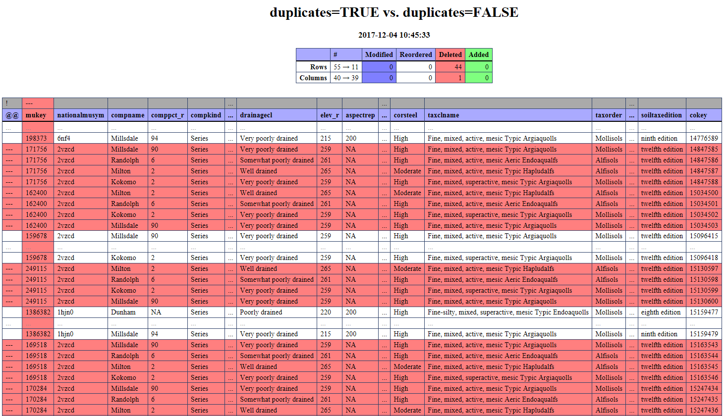
render_diff(d, title='duplicates=TRUE vs. duplicates=FALSE')

The two calls to get_component_from_SDA() generate the following SQL:

-- duplicates == TRUE
SELECT mukey, mu.nationalmusym, compname, comppct_r, compkind, majcompflag, localphase, slope_r, tfact, wei, weg, drainagecl, elev_r, aspectrep, map_r, airtempa_r, reannualprecip_r, ffd_r, nirrcapcl, nirrcapscl, irrcapcl, irrcapscl, frostact, hydgrp, corcon, corsteel, taxclname, taxorder, taxsuborder, taxgrtgroup, taxsubgrp, taxpartsize, taxpartsizemod, taxceactcl, taxreaction, taxtempcl, taxmoistscl, taxtempregime, soiltaxedition, cokey 
FROM legend l 
INNER JOIN
mapunit mu ON mu.lkey = l.lkey 
INNER JOIN (
SELECT compname, comppct_r, compkind, majcompflag, localphase, slope_r, tfact, wei, weg, drainagecl, elev_r, aspectrep, map_r, airtempa_r, reannualprecip_r, ffd_r, nirrcapcl, nirrcapscl, irrcapcl, irrcapscl, frostact, hydgrp, corcon, corsteel, taxclname, taxorder, taxsuborder, taxgrtgroup, taxsubgrp, taxpartsize, taxpartsizemod, taxceactcl, taxreaction, taxtempcl, taxmoistscl, taxtempregime, soiltaxedition, cokey , mukey AS mukey2 FROM component
) AS c ON c.mukey2 = mu.mukey 
WHERE muname = 'Millsdale silty clay loam, 0 to 2 percent slopes' 
ORDER BY cokey, compname, comppct_r DESC;

-- duplicates == FALSE
SELECT DISTINCT mu.nationalmusym, compname, comppct_r, compkind, majcompflag, localphase, slope_r, tfact, wei, weg, drainagecl, elev_r, aspectrep, map_r, airtempa_r,
 reannualprecip_r, ffd_r, nirrcapcl, nirrcapscl, irrcapcl, irrcapscl, frostact, hydgrp, corcon, corsteel, taxclname, taxorder, taxsuborder, taxgrtgroup, taxsubgrp, 
taxpartsize, taxpartsizemod, taxceactcl, taxreaction, taxtempcl, taxmoistscl, taxtempregime, soiltaxedition, cokey 
FROM legend l
INNER JOIN mapunit mu ON mu.lkey = l.lkey 
INNER JOIN (
	SELECT MIN(nationalmusym) nationalmusym2, MIN(mukey) AS mukey2 
	FROM mapunit
	GROUP BY nationalmusym
) AS mu2 ON mu2.nationalmusym2 = mu.nationalmusym 
INNER JOIN (
	SELECT compname, comppct_r, compkind, majcompflag, localphase, slope_r, tfact, wei, weg, drainagecl, elev_r, aspectrep, map_r, airtempa_r, reannualprecip_r, 
	ffd_r, nirrcapcl, nirrcapscl, irrcapcl, irrcapscl, frostact, hydgrp, corcon, corsteel, taxclname, taxorder, taxsuborder, taxgrtgroup, taxsubgrp, taxpartsize, 
	taxpartsizemod, taxceactcl, taxreaction, taxtempcl, taxmoistscl, taxtempregime, soiltaxedition, cokey , mukey AS mukey2 
	FROM component
) AS c ON c.mukey2 = mu2.mukey2 
WHERE muname = 'Millsdale silty clay loam, 0 to 2 percent slopes' 
ORDER BY cokey, compname, comppct_r DESC

The differences in results, truncated for clarity:

semi-corrupt data returned by fetchSCAN() queries

Every query to the SCAN / SNOTEL web-service returns an "extra" day on September 30th. This affects all sensors and all years.

automatic conversion of `texture_class` to factor

It would be useful to set the factor levels according to a logical sequence.

.formatLandformString() needs review

composite horizons

how should A/B horizons be dealt with when entered as 2 horizons sharing the same depths?

document NASIS queries required for extended query / veg results

We may need to explicitly state the NASIS queries required to satisfy:

SELECT siteiid, vegplotid, vegplotname, obsdate, primarydatacollector, datacollectionpurpose, assocuserpedonid, ppi.seqnum, plantsym, plantsciname, plantnatvernm, orderofdominance, speciescancovpct, speciescancovclass

  FROM site_View_1 AS s
  INNER JOIN siteobs_View_1 AS so ON so.siteiidref = s.siteiid
  LEFT JOIN vegplot_View_1 AS v on v.siteobsiidref = so.siteobsiid
  LEFT JOIN plotplantinventory_View_1 AS ppi ON ppi.vegplotiidref = v.vegplotiid
  LEFT OUTER JOIN plant ON plant.plantiid = ppi.plantiidref;

write functions for getting / processing NASIS text notes

phnaf moved out of phorizon and into phlabresults

need to add a query to the ext_data to pull this in or add a join to the phlabresults table to pull it into the phorizon query directly

Ensure that new rock fragment sorting code gives similar results as old code

The old code (SQL) may have missed some data that spanned multiple size classes.

Test:

library(soilDB)

# CRAN soilDB -- SQL based RF sorting
load('old-RF-code.rda')
# GH soilDB -- R based RF sorting
x.new <- fetchNASIS()

# sanity check: rows in same order?
# YES
all(x.old$phiid == x.new$phiid)


# compare proportion of differences old vs. new
prop.table(table(x.old$fine_gravel == x.new$fine_gravel))
prop.table(table(x.old$gravel == x.new$gravel))
prop.table(table(x.old$cobbles == x.new$cobbles))
prop.table(table(x.old$stones == x.new$stones))
prop.table(table(x.old$boulders == x.new$boulders))
prop.table(table(x.old$parafine_gravel == x.new$parafine_gravel))
prop.table(table(x.old$paragravel == x.new$paragravel))
prop.table(table(x.old$paracobbles == x.new$paracobbles))
prop.table(table(x.old$channers == x.new$channers))
prop.table(table(x.old$flagstones == x.new$flagstones))
prop.table(table(x.old$parachanners == x.new$parachanners))
prop.table(table(x.old$paraflagstones == x.new$paraflagstones))
prop.table(table(x.old$total_frags_pct == x.new$total_frags_pct))

# ... all are <= 1% differences

# compare magnitude of differences
sqrt(mean((x.old$fine_gravel - x.new$fine_gravel)^2, na.rm=TRUE)) # 2%
sqrt(mean((x.old$gravel - x.new$gravel)^2, na.rm=TRUE)) # 5%
sqrt(mean((x.old$cobbles - x.new$cobbles)^2, na.rm=TRUE)) # < 1%
sqrt(mean((x.old$total_frags_pct - x.new$total_frags_pct)^2, na.rm=TRUE)) # 0


# investigate differences in gravel
summary(x.old$gravel - x.new$gravel)

# ... new gravel volume is always smaller than old gravel

# investigate trouble horizons / pedons
idx <- which((x.old$gravel - x.new$gravel) > 5)
h.old <- horizons(x.old)[idx, c('peiid', 'phiid', 'hzname', 'fine_gravel', 'gravel', 'cobbles')]
h.new <- horizons(x.new)[idx, c('fine_gravel', 'gravel', 'cobbles', 'total_frags_pct')]

cbind(h.old, h.new)

p <- unique(h.old$peiid)
x.old$pedon_id[which(profile_id(x.old) %in% p)]

generalize get_metadata()

get_metadata() is defined in a couple of functions:

• uncode()
• .metadata_replace()

This function is typically followed by a if/else block which determines the source for "metadata":

 # load current metadata table
  if (NASIS == TRUE){
    metadata <- get_metadata()
  } else {
    load(system.file("data/metadata.rda", package="soilDB")[1])
  }

@smroecker : what do you think about abstracting this function into .get_metadata(NASIS) which then returns an object called metadata?

better documentation for fill argument to NASIS functions

See:

• get_component_horizon_data_from_NASIS_db()

NASIS surface rf summary should use soilDB::simplifyFragmentData()

This affects pedon and component queries.

some NASIS user site IDs interpreted as scientific notation

Try this one 056E916010:

library(soilDB)
x <- get_site_data_from_NASIS_db()

results:

'data.frame':	1 obs. of  38 variables:
 $ siteiid           : int 1353895
 $ peiid             : int 1245208
 $ site_id           : num Inf
 $ pedon_id          : num Inf
 $ obs_date          : POSIXct, format: "1991-06-27"
[...]

Notice site_id and pedon_id are interpreted as numbers in scientific notation that overflow limits of R's datatype.

I can't find any arguments to RODBC::sqlQuery() that might solve this problem.

figure out gen_hz field

Add dsp_comparable_layer_id to the phorizon queries....this is our gen_hz field.

??? Needs clarification.

should NASIS query functions target only the selected set?

Example from soilDB::get_component_data_from_NASIS_db():

SELECT dmudesc, compname, comppct_r, compkind, majcompflag, localphase, drainagecl, pmgroupname, elev_r, slope_l, slope_r, slope_h, aspectrep, map_r, airtempa_r as maat_r, soiltempa_r as mast_r, reannualprecip_r, ffd_r, tfact, wei, weg, nirrcapcl, nirrcapscl, irrcapcl, irrcapscl, frostact, hydgrp, corcon, corsteel, taxclname, taxorder, taxsuborder, taxgrtgroup, taxsubgrp, taxpartsize, taxpartsizemod, taxceactcl, taxreaction, taxtempcl, taxmoistscl, taxtempregime, soiltaxedition, coiid, dmuiid
  
  FROM 
  datamapunit_View_1 dmu INNER JOIN
  component co ON co.dmuiidref = dmu.dmuiid LEFT OUTER JOIN
  copmgrp ON copmgrp.coiidref = co.coiid AND copmgrp.rvindicator = 1

Discuss

Should queries like these (really, all queries to NASIS) limit selection to the special selected set "views"? Looking over the pedon and component code, I see a mixture of the two styles. There are a few cases where using the base tables (pedon vs. pedon_View_1) seems "correct":

• the first table in the query is joined to a base table via INNER join
• the base table isn't something that you can adjust via selected set, e.g. localplant or geomorfeattype

Other than that, there should be systematic use of one or the other. Using the base tables can be handy when one hasn't fully loaded the selected set. That road leads to inconsistency. I suggest using the selected set--with an option for hitting the base tables via lazy=TRUE.

functions querying local NASIS need flag for toggling selected set

multiple texture classes per horizon

how should multiple textures be dealt with? (2 rows/hz are currently returned)

• can this be fixed in SQL ?
• NASIS: we are keeping only the first record
• PedonPC: texture class is ommited from query

fetchOSD changes

• return parsed chunks from osd.fulltext2 [done]
• further parsing of drainage class in R code [done]
• MLRA overlap data (1:many)
• geomorphic summaries (1:many)
• series stats (1:1)
• parent material summaries (1:many)

consider changing default behavior of `fetchNASIS()`

It would probably be a good idea to error on the side of inclusion when loading pedons from NASIS:

change default argument rmHzErrors = TRUE to rmHzErrors = FALSE.

Note that setting rmHzErrors = FALSE will still result in a "check" with offending pedons printed as QC notes. (as of 195c67f)

switch to WGS84 coordinates when querying NASIS pedons

get_site_data_from_NASIS_db()

SDA_query updates

The new JSON+COLUMNAMES format is available:

https://sdmdataaccess.sc.egov.usda.gov/WebServiceHelp.aspx

Old version, XML:

post.data <- jsonlite::toJSON(list(query=q, format='xml'), auto_unbox = TRUE)

New version, JSON:
post.data <- jsonlite::toJSON(list(query=q, format='JSON+COLUMNNAME'), auto_unbox = TRUE)

After switching, it will be much simpler to process mutli-table queries, examples:

https://sdmdataaccess.sc.egov.usda.gov/documents/AdvancedQueries.html

Results are a character matrix:

$Table1
      [,1]      [,2]               
 [1,] "mukey"   "area"             
 [2,] "76183"   "450931.751630753" 
 [3,] "76184"   "28054.5407755375" 
 [4,] "86603"   "24981.4040058702" 
 [5,] "86605"   "7703.01425500028" 
 [6,] "86627"   "18289.0252154469" 
 [7,] "1697855" "958309.314945273" 

Therefore some work would be required to strip first line, convert to DF, and assign column names.

Changes will make it possible to use SDA_query() to generate a persistent AOI from arbitrary extent or sp object, then generate a link to WSS.

How do we get this to work:

q <- "-- A temporary table will hold the set of mapunit keys
~DeclareIntTable(@mukeyList)~
insert into @mukeyList
select  mu.mukey from legend L left join mapunit MU on L.lkey = MU.lkey
where L.areatypename = 'Non-MLRA Soil Survey Area' and L.areasymbol = 'ND053'
and mu.farmlndcl  = 'Farmland of statewide importance';
 
-- Define the AOI from the list of mapunits
~CreateAoiFromMukeyList(@mukeyList,@aoiid,@message)~
 
-- display the id number of the newly-created AOI.
select @aoiId [@aoiid]"

<ServiceException>
Invalid query: Incorrect syntax near &#39;~&#39;.
Must declare the scalar variable &quot;@aoiId&quot;.</ServiceException>

# reported by httr::stop_for_status()
Error: Bad Request (HTTP 400).

... Follow-up with Phil.

add check for same top and bottom horizon depths to fetchNASIS?

if top and bottom horizon depths have the same value, it creates an error in functions that subtract one from the other (divide by 0)
for example the aggregateColor function uses hxdepb-hzdept

consolidation of fetch/get functions

There are a couple main interfaces to our data, each with unique qualities:

• NASIS: request "everything" in the selected set, pedons / components / anything
• SDA: request is a fully-formed SQL statement, component data only, limits on result set size
• LIMS-WWW reports (NASIS remote server): requests are in the form of report URLs and parameters, severe limits on request and result size

Ideally, each interface gets its own function:

• fetchNASIS(): gains an argument to select pedons, components, vegdata, ... ?
• fetchSDA(): smarter than SDA_query() when geometry involved
• fetchLIMS: URLs hard-coded, user supplies parameters (?)

Why both changing the status quo? Well, there are now many functions spread across many files that all do very similar things. Consolidation is a good time to address open issues related to these functions. Also, this is a good opportunity to move away from manual decoding of coded values in SQL (fetchNASIS) to use of uncode().

Ideally these functions would do their best to return comparable data structures whenever possible.

use of data() in package

R CMD check --as-cran reports:

Found the following calls to data() loading into the global environment:
File 'soilDB/R/get_component_from_SDA.R':
  data(nasis_metadata, package = "soilDB")
File 'soilDB/R/uncode.R':
  data(nasis_metadata, package = "soilDB")
File 'soilDB/R/utils.R':
  data(nasis_metadata, package = "soilDB")

Here is how it is done in munsell2rgb:

# note: this is incompatible with LazyData: true
# load look-up table from our package
# This should be more foolproof than data(munsell) c/o PR
load(system.file("data/munsell.rda", package="aqp")[1])

This is a CRAN-safe way to load data from a package. Adjust as needed for soilDB.

NASIS lab data functions aren't working as expected

Do we need all three functions?

• get_phlabresults_data_from_NASIS_db()
• get_labpedon_data_from_NASIS_db()
• get_lablayer_data_from_NASIS_db()

TODO:

• review SQL
• wt. mean code for multiple samples / hz needs to be simplified
• what about samples that don't fit cleanly within a single horizon?
• why do some queries return all NA?
• documentation

SDA_query without IO

Hi Dylan~
I'm in the process of using your excellent soilDB package for some point extractions from SSURGO, but needed a SDA_query-like function without writing to disk. I worked one out, and thought I would share as an issue (in lieu of a pull request). Note that it uses tibbles, as opposed to data.frames... it will work just as well with data.frames, though. Hope you are well!

Best,
Kyle

SDA_query <- function (q) 
{
  if (!requireNamespace("httr", quietly = TRUE) |
      !requireNamespace("jsonlite", quietly = TRUE) |
      !requireNamespace("readr", quietly = TRUE)) 
    stop("please install the `httr`, `jsonlite`, and `readr` packages", 
         call. = FALSE)
  
  df <- httr::POST(url = "https://sdmdataaccess.sc.egov.usda.gov/tabular/post.rest", 
             body = list(query = q, format = "json+columnname") %>%
               jsonlite::toJSON(auto_unbox = TRUE)) %>%
    httr::stop_for_status() %>%
    httr::content(simplifyVector = T) %$%
    Table %>%
    tibble::as_tibble()

  colnames(df) <- df[1,]
  df <- df[-1,]
  
  df %<>%
    dplyr::mutate_all(.funs = funs(parse_guess))

  return(df)
  
}

finish NASIS component queries and return similar objects as pedon queries

TODO

1. complete re-write of original code [done]
2. finish adding functions / columns for fetchNASIS() parity
3. new tutorial explaining usage (#128)
4. fix old code that is now broken

soilDB::SDA_query() not encoding NA correctly

Example:

library(soilDB)
x <- get_cosoilmoist_from_SDA(WHERE = "mukey = '1395352'", impute = TRUE)
str(x)

Note the "NA" in results:

'data.frame':	52 obs. of  14 variables:
 $ nationalmusym: chr  "2ssrz" "2ssrz" "2ssrz" "2ssrz" ...
 $ muname       : chr  "Drummer silty clay loam, 0 to 2 percent slopes" "Drummer silty clay loam, 0 to 2 percent slopes" "Drummer silty clay loam, 0 to 2 percent slopes" "Drummer silty clay loam, 0 to 2 percent slopes" ...
 $ compname     : chr  "Drummer" "Drummer" "Drummer" "Drummer" ...
 $ comppct_r    : int  94 94 94 94 94 94 94 94 94 94 ...
 $ month        : Factor w/ 12 levels "January","February",..: 4 4 8 12 2 2 1 1 7 6 ...
 $ flodfreqcl   : Factor w/ 8 levels "Not_Populated",..: 2 2 2 2 2 2 2 2 2 2 ...
 $ pondfreqcl   : Factor w/ 8 levels "Not_Populated",..: 5 5 1 1 5 5 5 5 1 1 ...
 $ dept_l       : chr  "0" "0" "NA" "NA" ...
 $ dept_r       : chr  "0" "15" "NA" "NA" ...
 $ dept_h       : chr  "0" "30" "NA" "NA" ...
 $ depb_l       : chr  "0" "200" "NA" "NA" ...
 $ depb_r       : chr  "15" "200" "NA" "NA" ...
 $ depb_h       : chr  "30" "200" "NA" "NA" ...
 $ status       : Factor w/ 6 levels "Not_Populated",..: 3 5 1 1 3 5 3 5 1 1 ...
 - attr(*, "SDA_id")= chr "Table"

This is a problem in SDA_query().

SDA_query breaks when records span multiple lines

An example:

library(soilDB)
SDA_query("SELECT * from mutext WHERE mukey = '462528';")

Multi-line records are the "problem".

The associated data look something like this when written to a temp file:

V1|V2|V3|V4|V5|V6|V7|V8|V9
1/6/2005 12:00:00 AM|Miscellaneous notes|Storie|NA|"This Storie Index number was calculated by a soil scientist using criteria based on the University of California the 1978 publication "Storie Index Soil Rating", UC Cooperative Extension Special Publication 3203".|461845|1233465|995986|dmutext
1/6/2005 12:00:00 AM|Miscellaneous notes|Storie|NA|"This Storie Index number was calculated by a soil scientist using criteria based on the University of California the 1978 publication "Storie Index Soil Rating", UC Cooperative Extension Special Publication 3203".|461904|1233517|996031|dmutext
1/6/2005 12:00:00 AM|Miscellaneous notes|Storie|NA|"This Storie Index number was calculated by a soil scientist using criteria based on the University of California the 1978 publication "Storie Index Soil Rating", UC Cooperative Extension Special Publication 3203".|461931|1233536|996050|dmutext
1/6/2005 12:00:00 AM|Miscellaneous notes|Storie|NA|"This Storie Index number was calculated by a soil scientist using criteria based on the University of California the 1978 publication "Storie Index Soil Rating", UC Cooperative Extension Special Publication 3203".|461933|1233538|996052|dmutext
1/6/2005 12:00:00 AM|Miscellaneous notes|Storie|NA|"This Storie Index number was calculated by a soil scientist using criteria based on the University of California the 1978 publication "Storie Index Soil Rating", UC Cooperative Extension Special Publication 3203".|461979|1233577|996083|dmutext
1/6/2005 12:00:00 AM|Miscellaneous notes|Storie|NA|"This Storie Index number was calculated by a soil scientist using criteria based on the University of California the 1978 publication "Storie Index Soil Rating", UC Cooperative Extension Special Publication 3203".|461980|1233578|996084|dmutext
1/6/2005 12:00:00 AM|Miscellaneous notes|Storie|NA|"This Storie Index number was calculated by a soil scientist using criteria based on the University of California the 1978 publication "Storie Index Soil Rating", UC Cooperative Extension Special Publication 3203".|461997|1195308|991933|dmutext
8/7/2003 12:00:00 AM|Nontechnical description|SOI|NA|AgB=Amador gravelly loam, 0 to 8 percent slopes



 Amador soils make up 85 percent of the map unit.  This soil is on a hill.    The parent material

 consists of residuum weathered from rhyolite.  The runoff class is medium.  The depth to a

 restrictive feature is 4 to 14 inches to bedrock (paralithic). This soil is well drained.  The

 slowest soil permeability within a depth of 60 inches is moderate.  Available water capacity to a

 depth of 60 inches is very low, and shrink swell potential is low. Annual flooding is none, and

 annual ponding is none.  The minimum depth to a water table is greater than 6 feet.  The assigned Kw

 erodibility factor is .24.   It is nonirrigated land capability subclass 7e.    This component is

 not a hydric soil.



  Typical Profile:

   H1 - 0 to 6 inches; gravelly loam; very strongly acid.

   H2 - 6 to 13 inches; gravelly loam; very strongly acid.

   H3 - 13 to 16 inches; weathered bedrock; .|462528|959642|4040385|mutext
1/6/2005 12:00:00 AM|Miscellaneous notes|Storie|NA|"This Storie Index number was calculated by a soil scientist using criteria based on the University of California the 1978 publication "Storie Index Soil Rating", UC Cooperative Extension Special Publication 3203".|462528|959643|911760|dmutext
1/6/2005 12:00:00 AM|Miscellaneous notes|Storie|NA|"This Storie Index number was calculated by a soil scientist using criteria based on the University of California the 1978 publication "Storie Index Soil Rating", UC Cooperative Extension Special Publication 3203".|462529|959644|911761|dmutext

multiple RV component texture group records results in duplicate horizons/logic fail

Noticed today that I had inadvertently checked two texture groups as RV for one of my component horizons.

The component wouldn't load via fetchNASIS_component_data() due to failing test_hz_logic(). The reason why was not immediately obvious from my NASIS horizon table.

Multiple RVs results in the duplication/overlap AFTER loading from DB when compressing the chorizon texture group table down to the texture field within the component SPC.

Was handy that this happened, as otherwise it would have persisted in there until I ran the RV validation, but it might be helpful to catch "multiple RV" issues with a more informative error message.

Also, should there be safeguards to prevent duplication of a record because of a many-to-one compression gone bad? or one that is "intractable" without a human decision? I can't currently think of a case where duplicating would be desired behavior.

basic NA-filling for fetchHenry() / fetchSCAN() / CDEC_query()

Add an option to each of these functions for simple NA-filling by methods from the zoo (or similar) package.

Other ideas:

• https://cran.rstudio.com/web/packages/timetk/vignettes/TK00_Time_Series_Coercion.html

adjust all HTTP requests to follow Hadley's advice

https://cran.r-project.org/web/packages/httr/vignettes/api-packages.html

documentation for soilDB::uncode()

• when to use
• case sensitivity
• cached copy of metadata vs. local NASIS
• etc.

.rockFragmentSieve() needs to include all cementation classes

 [1] "noncemented"         "indurated"           "moderately cemented" "strongly cemented"   "weakly cemented"     "extremely weakly"   
 [7] "very weakly"         "very strongly"       "weakly"              "moderately"          "strongly"            "extremely strong"   
[13] "H"                   "S" 

change all HTTP requests to SoilWeb to HTTPS

Affected files:

R/fetchKSSL.R
R/fetchOSD.R
R/fetchRaCA.R
R/mapunit_geom_by_ll_bbox.R
R/seriesExtent.R
R/SSURGO_spatial_query.R

Test:

• 2-1
• 2-2