mmspide / anomalize

Tidy anomaly detection

anomalize

Tidy anomaly detection

anomalize enables a tidy workflow for detecting anomalies in data. The main functions are time_decompose(), anomalize(), and time_recompose(). When combined, it’s quite simple to decompose time series, detect anomalies, and create bands separating the “normal” data from the anomalous data.

Anomalize In 2 Minutes (YouTube)

Check out our entire Software Intro Series on YouTube!

Installation

You can install the development version with devtools or the most recent CRAN version with install.packages():

# devtools::install_github("business-science/anomalize")
install.packages("anomalize")

How It Works

anomalize has three main functions:

• time_decompose(): Separates the time series into seasonal, trend, and remainder components
• anomalize(): Applies anomaly detection methods to the remainder component.
• time_recompose(): Calculates limits that separate the “normal” data from the anomalies!

Getting Started

Load the tidyverse and anomalize packages.

library(tidyverse)
library(anomalize)

Next, let’s get some data. anomalize ships with a data set called tidyverse_cran_downloads that contains the daily CRAN download counts for 15 “tidy” packages from 2017-01-01 to 2018-03-01.

Suppose we want to determine which daily download “counts” are anomalous. It’s as easy as using the three main functions (time_decompose(), anomalize(), and time_recompose()) along with a visualization function, plot_anomalies().

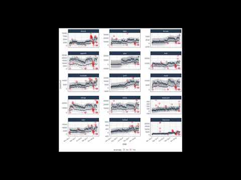
tidyverse_cran_downloads %>%
    # Data Manipulation / Anomaly Detection
    time_decompose(count, method = "stl") %>%
    anomalize(remainder, method = "iqr") %>%
    time_recompose() %>%
    # Anomaly Visualization
    plot_anomalies(time_recomposed = TRUE, ncol = 3, alpha_dots = 0.25) +
    labs(title = "Tidyverse Anomalies", subtitle = "STL + IQR Methods") 

Check out the anomalize Quick Start Guide.

Reducing Forecast Error by 32%

Yes! Anomalize has a new function, clean_anomalies(), that can be used to repair time series prior to forecasting. We have a brand new vignette - Reduce Forecast Error (by 32%) with Cleaned Anomalies.

tidyverse_cran_downloads %>%
    filter(package == "lubridate") %>%
    ungroup() %>%
    time_decompose(count) %>%
    anomalize(remainder) %>%
  
    # New function that cleans & repairs anomalies!
    clean_anomalies() %>%
  
    select(date, anomaly, observed, observed_cleaned) %>%
    filter(anomaly == "Yes")
#> # A time tibble: 19 x 4
#> # Index: date
#>    date       anomaly  observed observed_cleaned
#>    <date>     <chr>       <dbl>            <dbl>
#>  1 2017-01-12 Yes     -1.14e-13            3522.
#>  2 2017-04-19 Yes      8.55e+ 3            5202.
#>  3 2017-09-01 Yes      3.98e-13            4137.
#>  4 2017-09-07 Yes      9.49e+ 3            4871.
#>  5 2017-10-30 Yes      1.20e+ 4            6413.
#>  6 2017-11-13 Yes      1.03e+ 4            6641.
#>  7 2017-11-14 Yes      1.15e+ 4            7250.
#>  8 2017-12-04 Yes      1.03e+ 4            6519.
#>  9 2017-12-05 Yes      1.06e+ 4            7099.
#> 10 2017-12-27 Yes      3.69e+ 3            7073.
#> 11 2018-01-01 Yes      1.87e+ 3            6418.
#> 12 2018-01-05 Yes     -5.68e-14            6293.
#> 13 2018-01-13 Yes      7.64e+ 3            4141.
#> 14 2018-02-07 Yes      1.19e+ 4            8539.
#> 15 2018-02-08 Yes      1.17e+ 4            8237.
#> 16 2018-02-09 Yes     -5.68e-14            7780.
#> 17 2018-02-10 Yes      0.                  5478.
#> 18 2018-02-23 Yes     -5.68e-14            8519.
#> 19 2018-02-24 Yes      0.                  6218.

But Wait, There’s More!

There are a several extra capabilities:

• plot_anomaly_decomposition() for visualizing the inner workings of how algorithm detects anomalies in the “remainder”.

tidyverse_cran_downloads %>%
    filter(package == "lubridate") %>%
    ungroup() %>%
    time_decompose(count) %>%
    anomalize(remainder) %>%
    plot_anomaly_decomposition() +
    labs(title = "Decomposition of Anomalized Lubridate Downloads")

For more information on the anomalize methods and the inner workings, please see “Anomalize Methods” Vignette.

5-Minutes To Anomalize

Load libraries.

    library(tidyverse)
    library(tibbletime)
    library(anomalize)

Get some data. We’ll use the tidyverse_cran_downloads data set that comes with anomalize. A few points:

It’s a tibbletime object (class tbl_time), which is the object structure that anomalize works with because it’s time aware! Tibbles (class tbl_df) will automatically be converted.

It contains daily download counts on 15 “tidy” packages spanning 2017-01-01 to 2018-03-01. The 15 packages are already grouped for your convenience.

It’s all setup and ready to analyze with anomalize!

    tidyverse_cran_downloads
    #> # A time tibble: 6,375 x 3
    #> # Index:  date
    #> # Groups: package [15]
    #>    date       count package
    #>    <date>     <dbl> <chr>  
    #>  1 2017-01-01   873 tidyr  
    #>  2 2017-01-02  1840 tidyr  
    #>  3 2017-01-03  2495 tidyr  
    #>  4 2017-01-04  2906 tidyr  
    #>  5 2017-01-05  2847 tidyr  
    #>  6 2017-01-06  2756 tidyr  
    #>  7 2017-01-07  1439 tidyr  
    #>  8 2017-01-08  1556 tidyr  
    #>  9 2017-01-09  3678 tidyr  
    #> 10 2017-01-10  7086 tidyr  
    #> # … with 6,365 more rows

    tidyverse_cran_downloads_anomalized <- tidyverse_cran_downloads %>%
        time_decompose(count, merge = TRUE) %>%
        anomalize(remainder) %>%
        time_recompose()

    tidyverse_cran_downloads_anomalized %>% glimpse()
    #> Observations: 6,375
    #> Variables: 12
    #> Groups: package [15]
    #> $ package       <chr> "tidyr", "tidyr", "tidyr", "tidyr", "tidyr", "tidy…
    #> $ date          <date> 2017-01-01, 2017-01-02, 2017-01-03, 2017-01-04, 2…
    #> $ count         <dbl> 873, 1840, 2495, 2906, 2847, 2756, 1439, 1556, 367…
    #> $ observed      <dbl> 8.730000e+02, 1.840000e+03, 2.495000e+03, 2.906000…
    #> $ season        <dbl> -2761.4637, 901.0113, 1459.7147, 1429.7532, 1238.7…
    #> $ trend         <dbl> 5052.582, 5046.782, 5040.983, 5035.183, 5029.383, …
    #> $ remainder     <dbl> -1418.11842, -4107.79368, -4005.69726, -3558.93599…
    #> $ remainder_l1  <dbl> -3747.904, -3747.904, -3747.904, -3747.904, -3747.…
    #> $ remainder_l2  <dbl> 3707.661, 3707.661, 3707.661, 3707.661, 3707.661, …
    #> $ anomaly       <chr> "No", "Yes", "Yes", "No", "No", "No", "No", "No", …
    #> $ recomposed_l1 <dbl> -1456.786, 2199.890, 2752.793, 2717.032, 2520.278,…
    #> $ recomposed_l2 <dbl> 5998.779, 9655.454, 10208.358, 10172.597, 9975.843…

Equals:

    tt<-time_decompose(data=tidyverse_cran_downloads, count, merge = TRUE)
    dd<-anomalize(data=tt,remainder)
    tidyverse_cran_downloads_anomalized <- time_recompose(data=dd)
    glimpse(tidyverse_cran_downloads_anomalized)

We can use the general workflow for anomaly detection, which involves three main functions:

time_decompose(): Separates the time series into seasonal, trend, and remainder components anomalize(): Applies anomaly detection methods to the remainder component. time_recompose(): Calculates limits that separate the “normal” data from the anomalies!

Let’s explain what happened:

time_decompose(count, merge = TRUE): This performs a time series decomposition on the “count” column using seasonal decomposition. It created four columns: “observed”: The observed values (actuals) “season”: The seasonal or cyclic trend. The default for daily data is a weekly seasonality. “trend”: This is the long term trend. The default is a Loess smoother using spans of 3-months for daily data. “remainder”: This is what we want to analyze for outliers. It is simply the observed minus both the season and trend. Setting merge = TRUE keeps the original data with the newly created columns. anomalize(remainder): This performs anomaly detection on the remainder column. It creates three new columns: “remainder_l1”: The lower limit of the remainder “remainder_l2”: The upper limit of the remainder “anomaly”: Yes/No telling us whether or not the observation is an anomaly time_recompose(): This recomposes the season, trend and remainder_l1 and remainder_l2 columns into new limits that bound the observed values. The two new columns created are: “recomposed_l1”: The lower bound of outliers around the observed value “recomposed_l2”: The upper bound of outliers around the observed value We can then visualize the anomalies using the plot_anomalies() function.

    tidyverse_cran_downloads_anomalized %>%
        plot_anomalies(ncol = 3, alpha_dots = 0.25)

Equals:

    plot_anomalies(data=tidyverse_cran_downloads_anomalized, ncol = 3, alpha_dots = 0.25)

References

Several other packages were instrumental in developing anomaly detection methods used in anomalize:

• Twitter’s AnomalyDetection, which implements decomposition using median spans and the Generalized Extreme Studentized Deviation (GESD) test for anomalies.
• forecast::tsoutliers() function, which implements the IQR method.

Interested in Learning Anomaly Detection?

Business Science offers two 1-hour courses on Anomaly Detection:

• Learning Lab 18

  • Time Series Anomaly Detection with anomalize

• Learning Lab 17

  • Anomaly Detection with H2O Machine Learning