hiddensymmetries / simsopt

Simons Stellarator Optimizer Code

simsopt

simsopt is a framework for optimizing stellarators. The high-level routines of simsopt are in python, with calls to C++ or fortran where needed for performance. Several types of components are included:

• Interfaces to physics codes, e.g. for MHD equilibrium.
• Tools for defining objective functions and parameter spaces for optimization.
• Geometric objects that are important for stellarators - surfaces and curves - with several available parameterizations.
• Efficient implementations of the Biot-Savart law and other magnetic field representations, including derivatives.
• Tools for parallelized finite-difference gradient calculations.

The design of simsopt is guided by several principles:

• Thorough unit testing, regression testing, and continuous integration.
• Extensibility: It should be possible to add new codes and terms to the objective function without editing modules that already work, i.e. the open-closed principle. This is because any edits to working code can potentially introduce bugs.
• Modularity: Physics modules that are not needed for your optimization problem do not need to be installed. For instance, to optimize SPEC equilibria, the VMEC module need not be installed.
• Flexibility: The components used to define an objective function can be re-used for applications other than standard optimization. For instance, a simsopt objective function is a standard python function that can be plotted, passed to optimization packages outside of simsopt, etc.

simsopt is fully open-source, and anyone is welcome to use it, make suggestions, and contribute.

Several methods are available for installing simsopt. One recommended approach is to use pip:

pip install simsopt

For detailed installation instructions on some specific systems, see the wiki. Also, a Docker container is available with simsopt and its components pre-installed, which can be started using

docker run -it --rm hiddensymmetries/simsopt

More installation options, instructions for the Docker container, and other information can be found in the main simsopt documentation here.

Some of the physics modules with compiled code reside in separate repositories. These separate modules include

• VMEC, for MHD equilibrium.
• SPEC, for MHD equilibrium.
• booz_xform, for Boozer coordinates.

If you use simsopt in your research, kindly cite the code using this reference:

[1] M Landreman, B Medasani, F Wechsung, A Giuliani, R Jorge, and C Zhu, "SIMSOPT: A flexible framework for stellarator optimization", J. Open Source Software 6, 3525 (2021).

See also the simsopt publications page.

We gratefully acknowledge funding from the Simons Foundation's Hidden symmetries and fusion energy project.

simsopt's Issues

example/simsgeo not working

Hello Florian,

The simsgeo example in examples folder is not working. Could you please take a look at it? Please use the file in the tox branch.

Scalar minimization problem interface, similar to least_squares_serial_solve

Generic Optimizable interface class

For any external codes, we need an interface class to convert external class to Optimizable class.
Delineate the required properties and implement an interface that takes a function or class and generates Optimizable class. Replacement for Target class which was designed for previous implementation of Optimizable class.

Possible bug in test_mpi.py

Hello Matt,

I am wondering if there is a bug in https://github.com/hiddenSymmetries/simsopt/blob/master/tests/solve/test_mpi.py#L132

Fix API docs

API docs appear empty. Read The Docs build log shows a bunch of errors, which are probably related.

File missing

In the folder NCSX_test_data, the file NCSX_coil_coeffs.dat referred to by tests/geo/surface_test_helpers.py is missing. I am wondering how the tests are passing such as those in tests/geo/test_boozersurface.py

VMEC python module error

I attempted to install VMEC python wrapper with cmake on our cluster GADI.

I encounter the following error when I try to run the simsopt unit tests.

test_init_from_file (mhd.test_vmec.VmecTests) ... STOP allocation error in fixaray: istat2

It seems some error is encountered during memory allocated. To make sure it is not a problem of memory size, I have asked for 240G of memory, which should be sufficient. Has anyone encountered similar problems before? Any suggestions?

The compiler is GCC 8.3. The modules I have used are

1) pbs   2) intel-mkl/2019.3.199   3) python3/3.7.4   4) netcdf/4.7.3(default)   5) openmpi/4.0.3   6) cmake/3.18.2

Name error in simsgeo

I found there is a name error StelleratorSymmetricCylindricalFourierCurve in simsgeoapp or simsgeo that crashes the code. It should be StellaratorSymmetricCylindricalFourierCurve.

Bug in surface_test_helpers.py

Hello Florian,

Could you please take a look at line 71 in tests/geo/surface_test_helpers.py file? Next to raise there should be an exception. Instead, there is a string.

Put C++ class definition in header files

@florianwechsung ,

Regarding simsgeocpp, I am wondering about the logic behind the unconventional way of defining the C++ classes in cpp files. Is there any limitation you encountered for defining the classes in header files and implementing the class methods in the corresponding cpp files? If not, could you please put the class definitions in header files and include only the header files in the cpp files? Small methods (one or two lines) are typically defined as inline methods in the class definition and so they also can be moved to header file if you want. You can keep the implementation of the rest of the class methods in the cpp files.

Bharat

Summer and Multiplier for Optimizable objects

Problem

If we want to optimize J(a, b, c) = f(a, b) + g(b, c), then neitherf.x nor g.x really contains the full optimization space, so it would be good to have an object that combines the two, so that J.x contains a, b and c. In addition to combining all the optimizables, it would also simply expression objectives such as Flux([coil_1, coil_2]) + CurveLength(coil1) + CurveLength(coil2), and avoid the user having to do the summation by hand.

Demo Code

from simsopt.geo.curveobjectives import CurveLength, MinimumDistance
import numpy as np
import sys
import os
sys.path.append(os.path.join("..", "..", "tests", "geo"))
from surface_test_helpers import get_ncsx_data
curves, currents, ma = get_ncsx_data(Nt_coils=1)
J1 = CurveLength(curves[0])
J2 = CurveLength(curves[1])
J3 = MinimumDistance(curves, 1.0)
print(J1.J() + 2*J2.J() + J3.J())
J = J1 + 2.*J2 + J3
J.x # should contain np.concatenate((curves[0].x, curves[1].x, curves[2].x))
J.J() # should be equivalent to J1.J() + 2*J2.J() + J3.J()

Delete Optimizable properties that have dofs and state in the name

The above mentioned properties are synonymous to x and felt not needed by other team members. Delete them to provide a simple interface.

"Concepts" section on Magnetic fields and Biot Savart in the documentation

List of magnetic field classes

Here is a list of possible magnetic field classes that could be included in the magneticfieldclasses.py file:

• Reiman Model: see Appendix D of https://arXiv.org/pdf/2102.04497
• Dommaschk Potentials: see W. Dommaschk (1986), "Representations for vacuum potentials in stellarators", Comp. Phys. Comm. 40 (link)
• PointDipole: see equation 14 of https://arxiv.org/pdf/2009.06535

Add interface to DFO-LS

The work by @lindonroberts and Cora Cartis on Derivative Free optimization routines for least squares problems has been cleaning up prizes in the Numerical Analysis / Optimisation community recently. The stuff in scipy is all pretty old, so maybe we should add an interface to this solver.

https://github.com/numericalalgorithmsgroup/dfols

Delete DOF class

The current DOF class is not serving any purpose. Remove it.

Stochastic stage-2 coil optimization

It would be great to have the capability fully within simsopt to do the stage-2 problem (vary coil shapes to minimize \int (B dot n)^2 dS + regularization terms for a fixed target plasma boundary) with derivative-based stochastic optimization. No code can do this now, and this would basically combine the best features of FOCUS, DONSET, and pyPlasmaOpt. We basically have all the pieces for this, though some are now in pyPlasmaOpt. In practice, stellarator facility design activities these days use the 2-stage approach. So if we can demonstrate stochastic derivative-based stage-2 optimization, this would be a very useful tool for practical design.

Bug in advanced example

Please fix the os import bug in https://github.com/hiddenSymmetries/simsopt/blob/master/examples/3_Advanced/optimize_qs_and_islands_simultaneously.py

Also please add it to the github integrated tests so it runs when both vmec and spec are installed

Mayavi vs Pyvista, from the docker standpoint

I'm doing my JOSS review out of the provided Docker image and I'm just lamenting the fact that Mayavi keeps crashing my Jupyter server.

From what I can tell, it seems that Mayavi is used only in these two locations:

simsopt/src/simsopt/geo/surface.py

Lines 21 to 50 in 77c32e0

	def plot(self, ax=None, show=True, plot_normal=False, plot_derivative=False, scalars=None, wireframe=True):
	"""
	Plot the surface using mayavi.
	Note: the `ax` and `show` parameter can be used to plot more than one surface:
	.. code-block::
	ax = surface1.plot(show=False)
	ax = surface2.plot(ax=ax, show=False)
	surface3.plot(ax=ax, show=True)
	"""
	gamma = self.gamma()
	from mayavi import mlab
	mlab.mesh(gamma[:, :, 0], gamma[:, :, 1], gamma[:, :, 2], scalars=scalars)
	if wireframe:
	mlab.mesh(gamma[:, :, 0], gamma[:, :, 1], gamma[:, :, 2], representation='wireframe', color=(0, 0, 0), opacity=0.5)
	if plot_derivative:
	dg1 = 0.05 * self.gammadash1()
	dg2 = 0.05 * self.gammadash2()
	mlab.quiver3d(gamma[:, :, 0], gamma[:, :, 1], gamma[:, :, 2], dg1[:, :, 0], dg1[:, :, 1], dg1[:, :, 2])
	mlab.quiver3d(gamma[:, :, 0], gamma[:, :, 1], gamma[:, :, 2], dg2[:, :, 0], dg2[:, :, 1], dg2[:, :, 2])
	if plot_normal:
	n = 0.005 * self.normal()
	mlab.quiver3d(gamma[:, :, 0], gamma[:, :, 1], gamma[:, :, 2], n[:, :, 0], n[:, :, 1], n[:, :, 2])
	if show:
	mlab.show()

simsopt/src/simsopt/geo/curve.py

Lines 140 to 149 in af23454

	@requires(mlab is not None, "plot_mayavi requires mayavi")
	def plot_mayavi(self, show=True):
	"""
	Plot the curve using :mod:`mayavi.mlab` rather than :mod:`matplotlib.pyplot`.
	"""
	g = self.gamma()
	mlab.plot3d(g[:, 0], g[:, 1], g[:, 2])
	if show:
	mlab.show()

I suspect that if this was (simply, it looks like) rewritten using PyVista, we could then take advantage of https://docs.pyvista.org/extras/docker.html and get this to work from within the notebook! Is there anything I'm missing here? In particular, is there any tighter coupling/investment between Simsopt and Mayavi that I'm missing?

---

Of course, the whole issue of running this out of a Docker container is a side effect of SPEC being private, and the Docker image being the only way I can get my hands on it for review purposes - but that's a rant that I don't want to get into 😅

---

Let me add that this should in no way be considered a blocker for the JOSS review. Just putting the idea out there.

Move MPILogger code to simsopt

Because MPILogger is not hosted on pypi, pypi is rejecting simsopt uploads. MPILogger package is a single file with a permissive license. Add the file to simsopt with license on top of it.

Convert qsc example to graph framework

The qsc example in 2_Intermediate is using the old framework and needs to be modified to use the new graph based framework. However, the PyQSC codebase is mirroring the logic of the soon to be deprecated optimizable framework in simsopt. Do we work on this only from simsopt side or is PyQSC going to be modified?

Docker container containing SIMSOPT + SPEC + VMEC

VMEC2000 seems non-trivial to install, so it would greatly simplify things if we had a docker container with an installation of simsopt with all external codes

SPEC build failing in CI for pull requests.

Investigate the failure to import SPEC repo for pull requests.

Stage 2 Coil optimisation example

In coil optimisation we often have the case that we have a small number of coils (say 3) that is rotated and flipped to obtain a full stellarator. Currently we express this in the following form:

base_coils = get_coils(...) # these are 3 coils that we optimise for
base_currents = [...] # the three currents
stellarator = CoilCollection(base_coils, base_currents, nfp=3, stellsym=True)

full_coils = stellarator.coils
full_currents = stellarator.currents

the CoilCollection object takes care of the rotation and flipping of coils via RotatedCurve.
The dof/optimizable class should be able to deal with the following problem:

We have an objective that takes a list of coils and currents

J = SomeObjective(full_coils, full_currents)

and then we want to do the optimisation over base_coils and base_currents.

Give a high level overview in the README.md

Visualization optional dependencies

I see Mayavi is used for plotting e.g. here: https://simsopt.readthedocs.io/en/latest/simsopt.geo.html#simsopt.geo.surface.Surface.plot

However, the Docker container does not include it. Would it perhaps make sense to add somewhere around

simsopt/setup.cfg

Lines 62 to 69 in b3f3c31

	[options.extras_require]
	SPEC =
	py_spec >= 3.0.1
	pyoculus >= 0.1.1
	h5py >= 3.1.0
	f90nml >= 1.2
	MPI =
	mpi4py >= 3.0.3

a list of visualization package (matplotlib, mayavi, have I missed anything?) versions that work with the rest of the package?

Of course, I know mayavi can be a tough cookie to install due to its heavy VTK dependency. Matplotlib, at least, could be good candidate for now, especially for inclusion into the Docker image.

Whatcha think? :)

VMEC module naming

The names in the VMEC moduel can be optimized fto make end users life easy.
For example importing simsopt/modules/VMEC/vmec_class.py:VMEC class would be like

from simsopt.modules.VMEC.vmec_class import VMEC

1. You can see there are repetitions of vmec.
2. CAPS for folders and files is not a good idea. Its a pain to type CAPS. I am going to use lower case for the folder names.
3. Lets use __init__.py to shorten the import statement.
4. vmec_class.py will be renamed as core.py

Refer to #6 pull request

@requires decorator confuses sphinx

When the docs have a link to a class, using e.g.

:obj:`simsopt.util.mpi.MpiPartition`

the link does not work if the class has the @requires decorator. I noticed this problem in particular for the links to MpiPartition in
https://simsopt.readthedocs.io/en/latest/concepts.html#mpi-partitions-and-worker-groups
If the @requires decorator is removed from MpiPartition, the links in the docs work again.

DOF Data handling between C++ side and DOFs panda data frame class

Come up with a scheme where DOFs panda frame class can handle data sharing between C++ classes.

Automatic increase of Docker memory through specification in image file?

Investigate the possibility.

Modify caching implementation for Optimizable object

At present, Optimizable class implements caching by using a boolean variable to denote a new input is present. With this approach, all the objective functions in an Optimizable class are evaluated whenever a new input is supplied. And the results are stored in the cache. If one of the objective functions is called again, the cached value is used. This has the drawback of possibly requiring expensive evaluations of all objective functions even if most of them are not needed for a given problem.

Alternative implementations:

1. Use a separate boolean variable to denote new input for all objective functions. A new input sets all the variables for the objective functions. Whenever one of the objective functions is called, the called function refers to its own variable to either return the cache or do a calculation and update the cache. To minimize the workload on the developers, develop a method decorator that can handle this automatically, so that developers of objective functions don't have to deal with caching at all.
   Drawback: In addition to the cache, another set of variables have to be used.
   Pros: No need to deal with cache for new inputs, which could be costly.
2. Alternatively, don't use boolean variables to denote new_x. Instead, invalidate cache, whenever a new input is given. When an objective function is called, cache is checked and if not in a valid state, the function is computed and cache is updated.
   Drawback: Invalidating (deleting) and rebuilding cache could be costly in terms of memory operations..
   Pros: No need to store any additional variables.

Git submodules and python source distribution are not compatible

Hello Florian,

When creating a source distribution of simsopt, it is not possible to include .git file. Hence the git submodule feature won't work if someone uses the source distribution from pypi to install simsopt. Instead could you use FetchContent feature of CMake.

This was a snippet of CMake code I was using for one of my projects.

include(FetchContent)

FetchContent_DECLARE(
	yaml_cpp
	GIT_REPOSITORY	https://github.com/jbeder/yaml-cpp.git
)

You could google more about it.

Bharat

Some questions regarding profiling.cpp

@florianwechsung, @landreman

Hello Florian,

I am not fully familiar with the purpose of the profiling executable generated during the building of simsopt. Is it only to profile the speed of the C++ code? Or do you want it to be part of the distribution?

At present, profiling is a mandatory target in the CMakeLists. If it is only for profiling the C++ code and should be limited to developers, could you please make it an optional target?

Profiling.cpp is not part of the source distribution and so, installing simsopt from sdist zip is failing to build (because profiling is a mandatory target). I'll fix it by adding profiling.cpp to MANIFEST.in. But if you make it an optional target, we don't have to make it part of the sdist.

Finally regarding the location of profiling.cpp:
I am thinking of moving profiling/profiling.cpp to src/simsgeopp if you want it keep it a mandatory target. If it is an optional build, then we can keep the current layout or move the profiling folder to src folder to prevent an excessive number of folders at the root level.

code coverage

Auto versioning the code

The current manual increment of the version string is not feasible in the long run. Instead, investigate tools like bumpversion and versioneer to increment the version.

Remove all print statements from the main code base

All printing should be done via the logging facilities so that messages such as

No module named 'vmec'
No module named 'spec'
No module named 'py_spec'
No module named 'pyoculus'
No module named 'booz_xform'

or

The given Optimizable object is already a parent

don't pollute user output.

clean up examples folder

• Group into folders
• have input files in subfolders

dof ordering typo

The description of the dof ordering on this line

simsopt/src/simsoptpp/curvexyzfourier.h

Line 17 in 6977128

[x_{c,0},...,x_{c,order},x_{s,1},...,x_{s,order},y_{c,0},....]

is inaccurate. The ordering is actually

xc0, xs1, xc1, xs2, xc2,..., yc0, ys1, yc1, ys2, yc2, ..., zc0, zs1, zc1, zs2, zc2, ...

I haven't checked the other geometry classes, but we should check them to make sure they are correct.

High level overview for simsopt.geo in the documentation

Use boost when building the simsopt wheel

For particle tracing to work, simsopt needs to be compiled with boost. This requires boost to be installed on the manylinux image.

TODO Items

1. Install boost on manylinux image
2. Use that image to build wheels.

Fix typos in the doc

Just found that there are some typos in the documentation. On https://simsopt.readthedocs.io/en/latest/getting_started.html#installation, the two installation lines are identical and should use --user. I don't know the correct commands, otherwise, I can create a PR myself.

If you want to build SIMSOPT locally with the optional dependencies, you can run

pip install –user -e .[MPI,SPEC]

However, if you’re using a zsh terminal (example: latest Macbook versions), you’ll need to run instead

pip install –user -e .[MPI,SPEC]

Installation error on macbook

Hi, I am trying to install SIMSOPT on my macbook using GCC-10. I mannually set $CC and $CXX to be directed to GCC execubables. After I ran pip install -e .[MPI,SPEC], no errors show up. (I will get errors if I didn't specify $CC, $CXX.)

But when I tried to import simsopt, I got the following error, which is probably caused by the pybind.

In [1]: import simsopt                                                                                                                                                                                                                                                                                              
---------------------------------------------------------------------------
RuntimeError                              Traceback (most recent call last)
RuntimeError: module compiled against API version 0xe but this version of numpy is 0xd
---------------------------------------------------------------------------
ImportError                               Traceback (most recent call last)
<ipython-input-1-ff876a4d7849> in <module>
----> 1 import simsopt

~/Documents/Codes/simsopt/src/simsopt/__init__.py in <module>
     20 
     21 from ._core import make_optimizable
---> 22 from .objectives import LeastSquaresTerm, LeastSquaresProblem
     23 from .solve import least_squares_serial_solve
     24 from .util import initialize_logging

~/Documents/Codes/simsopt/src/simsopt/objectives/__init__.py in <module>
----> 1 from .least_squares import LeastSquaresTerm, LeastSquaresProblem
      2 
      3 __all__ = ['LeastSquaresTerm', 'LeastSquaresProblem']

~/Documents/Codes/simsopt/src/simsopt/objectives/least_squares.py in <module>
     17 from scipy.optimize import least_squares
     18 
---> 19 from .._core.dofs import Dofs
     20 from .._core.util import isnumber
     21 from .._core.optimizable import function_from_user, Target

~/Documents/Codes/simsopt/src/simsopt/_core/dofs.py in <module>
     15 
     16 from .optimizable import function_from_user
---> 17 from .util import unique, ObjectiveFailure, finite_difference_steps
     18 
     19 logger = logging.getLogger(__name__)

~/Documents/Codes/simsopt/src/simsopt/_core/util.py in <module>
     16 
     17 from ..util.types import RealArray
---> 18 from simsoptpp import Curve   # To obtain pybind11 metaclass
     19 
     20 

ImportError: SystemError: <built-in method __contains__ of dict object at 0x7ffc35657180> returned a result with an error set

After searching the internet, it looks there is some solutions (link), but the commits is not simple. Has anyone saw this before?

More granular testing and documentation of RegularGridInterpolant

`set_points` should check on the python side that the array is C contiguous and give a useful error message if not

Bug in mpi_solve.py

Hello Matt,

There is a bug in mpi_solve.py at line 209. The prob variable was not defined anywhere in that scope. Could you please fix it and write a test case that covers that part of the code?

Thank you,
Bharat

Garbage collection of Optimizable objects

Due to the double link between parent and child Optimizable objects, Optimizable objects are not garbage collected even when they go out of scope.

Explore weak references as suggested by Florian and custom delete methods to facilitate garbage collection.

Many C++ methods have no description in docs

There are a bunch of methods defined in C++, such as gamma() for surfaces and curves, that do not have any description in the API docs, or when a user uses help().

Detect cycles in the new graph based optimizable framework

A user could create a cycle in the optimization graph unknowingly using the current mechanism.

Implement a mechanism to detect cycles.

Segmentation fault with multi-volume SPEC equilibria

Hello!

I am trying to run simsopt to optimize some SPEC equilibria and I am running into some bugs I don't know how to solve. Note that I am new to python so it is very likely that some of these "bugs" are introduced by myself... Nevertheless, I would appreciate if someone could help me understand what is going on.

So, let me first say that I installed simsopt and SPEC py_wrappers, and it seems to work fine - I was able to run the example simsopt/examples/2_Intermediate/eliminate_magnetic_islands.py.

Now, I want to do the same kind of optimization but with a multi-volume, finite beta SPEC equilibrium (input file:
Input_000.txt). I tried to generate a Spec object and to run SPEC with the following script:

import logging
from simsopt.mhd.spec import Spec

logging.basicConfig(filename='loggerOutput.log', level=logging.DEBUG)

s = Spec('Input_000.sp')

s.run()

This doesn't seem to work - I get a segmentation fault. Terminal output:

(simsopt) abaillod@spcpc602:~/Physics/Optimization/RotatingEllipse/FixedBoundary/BoundaryOptimization/test> python test.py
No module named 'vmec'
readin :            : 
readin : ********** : Igeometry=  3 ; Istellsym=  1 ; Lreflect=  0 ;
readin :            : Lfreebound=  0 ; phiedge=  1.000000000000000E+00 ; curtor=  0.000000000000000E+00 ; curpol=  0.000000000000000E+00 ;
readin :            : gamma=  0.000000000000000E+00 ;
readin :            : Nfp=  5 ; Nvol=  8 ; Mvol=  8 ; Mpol=  6 ; Ntor=  4 ;
readin :            : pscale=  1.00000E+00 ; Ladiabatic= 0 ; Lconstraint=  3 ; mupf: tol,its=  1.00E-12 , 128 ;
readin :            : Lrad = 12, 6, 6, 6, 6, 6, 6, 6,
readin :            : 
readin : ********** : Linitialize=  0 ;LautoinitBn=  1 ; Lzerovac= 0 ; Ndiscrete= 2 ;
readin :            : Nquad=  -1 ; iMpol=  -4 ; iNtor=  -4 ;
readin :            : Lsparse= 0 ; Lsvdiota= 0 ; imethod= 3 ; iorder= 2 ; iprecon= 1 ; iotatol= -1.00000E+00 ;
readin :            : Lextrap= 0 ; Mregular= -1 ; Lrzaxis= 2 ; Ntoraxis= 3 ;
readin :            : 
readin : ********** : LBeltrami= 4 ; Linitgues= 1 ; Lmatsolver= 3 ; LGMRESprec= 1 ; NiterGMRES= 200 ; epsGMRES=  1.00000E-14 ; epsILU=  1.00000E-12 ;
readin :            : 
readin : ********** : Lfindzero= 2 ;
readin :            : escale=  0.00000E+00 ; opsilon=  1.00000E+00 ; pcondense=  4.000 ; epsilon=  1.00000E+00 ; wpoloidal= 1.0000 ; upsilon=  1.00000E+00 ;
readin :            : forcetol=  1.00000E-12 ; c05xmax=  1.00000E-06 ; c05xtol=  1.00000E-12 ; c05factor=  1.00000E-04 ; LreadGF= T ; 
readin :            : mfreeits=   0 ; gBntol=  1.00000E-06 ; gBnbld=  6.66000E-01 ;
readin :            : vcasingeps=  1.00000E-12 ; vcasingtol=  1.00000E-08 ; vcasingits=     8 ; vcasingper=     1 ;
readin :            : 
readin : ********** : odetol=  1.00E-07 ; nPpts=     0 ;
readin :            : LHevalues= F ; LHevectors= F ; LHmatrix= F ; Lperturbed= 0 ; dpp= -1 ; dqq= -1 ; dRZ=  1.00000000E-05 ; Lcheck=  0 ; Ltiming= F ;
readin :            : 
readin :            : myid=  0 ; Rscale= 1.000000000000000E+01 ;
preset :            : myid=  0 ; Mrad= 12 : Lrad= 12,  6,  6,  6,  6,  6,  6,  6,
preset : ********** : LBsequad= F , LBnewton= F , LBlinear= T ;
preset :            : 
preset : ********** : Nquad=  -1 ; mn=   59 ; NGdof=   819 ; NAdof=   705,   768,   768,   768,   768,   768,   768,   768,
preset :            : 
preset : ********** : Nt=    48 ; Nz=    32 ; Ntz=     1536 ;
In __init__, si.istellsym= 1  stellsym= True
In run, si.istellsym= 1  stellsym= True
readin :            : 
readin : ********** : Igeometry=  3 ; Istellsym=  1 ; Lreflect=  0 ;
readin :            : Lfreebound=  0 ; phiedge=  1.000000000000000E+00 ; curtor=  0.000000000000000E+00 ; curpol=  0.000000000000000E+00 ;
readin :            : gamma=  0.000000000000000E+00 ;
readin :            : Nfp=  5 ; Nvol=  8 ; Mvol=  8 ; Mpol=  6 ; Ntor=  4 ;
readin :            : pscale=  1.00000E+00 ; Ladiabatic= 0 ; Lconstraint=  3 ; mupf: tol,its=  1.00E-12 , 128 ;
readin :            : Lrad = 12, 6, 6, 6, 6, 6, 6, 6,
readin :            : 
readin : ********** : Linitialize=  0 ;LautoinitBn=  1 ; Lzerovac= 0 ; Ndiscrete= 2 ;
readin :            : Nquad=  -1 ; iMpol=  -4 ; iNtor=  -4 ;
readin :            : Lsparse= 0 ; Lsvdiota= 0 ; imethod= 3 ; iorder= 2 ; iprecon= 1 ; iotatol= -1.00000E+00 ;
readin :            : Lextrap= 0 ; Mregular= -1 ; Lrzaxis= 2 ; Ntoraxis= 3 ;
readin :            : 
readin : ********** : LBeltrami= 4 ; Linitgues= 1 ; Lmatsolver= 3 ; LGMRESprec= 1 ; NiterGMRES= 200 ; epsGMRES=  1.00000E-14 ; epsILU=  1.00000E-12 ;
readin :            : 
readin : ********** : Lfindzero= 2 ;
readin :            : escale=  0.00000E+00 ; opsilon=  1.00000E+00 ; pcondense=  4.000 ; epsilon=  1.00000E+00 ; wpoloidal= 1.0000 ; upsilon=  1.00000E+00 ;
readin :            : forcetol=  1.00000E-12 ; c05xmax=  1.00000E-06 ; c05xtol=  1.00000E-12 ; c05factor=  1.00000E-04 ; LreadGF= T ; 
readin :            : mfreeits=   0 ; gBntol=  1.00000E-06 ; gBnbld=  6.66000E-01 ;
readin :            : vcasingeps=  1.00000E-12 ; vcasingtol=  1.00000E-08 ; vcasingits=     8 ; vcasingper=     1 ;
readin :            : 
readin : ********** : odetol=  1.00E-07 ; nPpts=     0 ;
readin :            : LHevalues= F ; LHevectors= F ; LHmatrix= F ; Lperturbed= 0 ; dpp= -1 ; dqq= -1 ; dRZ=  1.00000000E-05 ; Lcheck=  0 ; Ltiming= F ;
readin :            : 
Segmentation fault (core dumped)

And the file loggerOutput.log:

INFO:simsopt.mhd.spec:Initializing a SPEC object from file: Input_000.sp
DEBUG:simsopt.mhd.spec:Entering init
DEBUG:simsopt.mhd.spec:Done with initialize_inputs
DEBUG:simsopt.mhd.spec:Done with read_inputlists_from_file
DEBUG:simsopt.mhd.spec:About to call broadcast_inputs
DEBUG:simsopt.mhd.spec:About to call preset
DEBUG:simsopt.mhd.spec:Done with init
INFO:simsopt.mhd.spec:Preparing to run SPEC.
INFO:simsopt.mhd.spec:Running SPEC using filename Input_000_000_000000
DEBUG:simsopt.mhd.spec:About to call check_inputs
DEBUG:simsopt.mhd.spec:About to call broadcast_inputs
DEBUG:simsopt.mhd.spec:About to call preset

I am not sure if this problem is related to SIMSOPT or to SPEC python wrappers though. Any help would be appreciated!

Thank you!

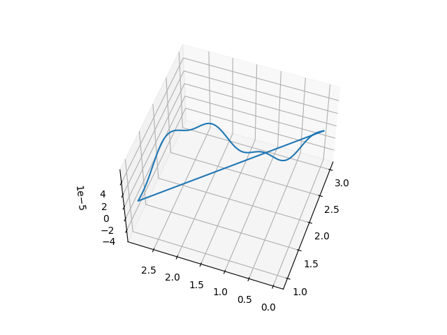
`minimize_curve_length.py` example does not converge to a circle?

To quote:

Minimize the length of a curve, holding the 0-frequency Fourier mode fixed.
The result should be a circle.

I ran the example using the provided Docker image with simsopt.__version__ being 0.4.0, in a Jupyter notebook, then plotted the curve using

%pip install matplotlib
%matplotlib notebook
curve.plot()

It doesn't seem to be particularly circular, no mater how I rotate it! 😉

Print-out from the execution

WARNING:absl:No GPU/TPU found, falling back to CPU. (Set TF_CPP_MIN_LOG_LEVEL=0 and rerun for more info.)

Initial curve dofs:  [ 3.         -0.47167117 -0.14711749 -0.36173382 -0.12887794 -0.19145344
  0.37352108  0.18049693  0.34338664]
Initial curve length:  47.51029349787225
finite difference Jacobian:
[[ -4.16447993   1.08533634 -31.92883693 -17.17364281  -2.05079456
   10.62181397   9.67475973  49.24442454]]
Analytic Jacobian:
[[ -4.16447995   1.08533638 -31.92883691 -17.17364278  -2.05079457
   10.62181394   9.67475967  49.24442449]]
Difference:
[[ 2.91588123e-08 -4.27509244e-08 -1.22633423e-08 -3.29675203e-08
   1.17619621e-08  2.69913691e-08  6.07857036e-08  5.03375546e-08]]
   Iteration     Total nfev        Cost      Cost reduction    Step norm     Optimality   
       0              1         1.1286e+03                                    2.34e+03    
       1              2         6.8936e+02      4.39e+02       8.47e-01       2.22e+03    
       2              4         3.3791e+02      3.51e+02       2.12e-01       8.36e+02    
       3              6         2.6535e+02      7.26e+01       1.06e-01       3.18e+02    
       4              7         2.1860e+02      4.68e+01       2.12e-01       4.04e+02    
       5              9         2.0364e+02      1.50e+01       5.30e-02       1.42e+02    
       6             10         1.9599e+02      7.65e+00       5.30e-02       1.22e+02    
       7             11         1.8839e+02      7.60e+00       1.06e-01       2.24e+02    
       8             13         1.8439e+02      3.99e+00       2.65e-02       7.46e+01    
       9             14         1.8260e+02      1.80e+00       2.65e-02       6.38e+01    
      10             15         1.8185e+02      7.42e-01       5.30e-02       1.76e+02    
      11             16         1.8009e+02      1.77e+00       1.32e-02       7.56e+01    
      12             17         1.7944e+02      6.47e-01       1.32e-02       3.88e+01    
      13             18         1.7896e+02      4.76e-01       1.32e-02       3.31e+01    
      14             19         1.7864e+02      3.20e-01       2.65e-02       7.94e+01    
      15             21         1.7825e+02      3.91e-01       6.62e-03       2.95e+01    
      16             22         1.7812e+02      1.38e-01       6.62e-03       1.97e+01    
      17             23         1.7800e+02      1.12e-01       6.62e-03       1.70e+01    
      18             24         1.7792e+02      8.26e-02       6.62e-03       1.75e+01    
      19             25         1.7787e+02      5.47e-02       6.62e-03       2.14e+01    
      20             26         1.7783e+02      4.07e-02       6.62e-03       2.28e+01    
      21             27         1.7779e+02      3.38e-02       1.66e-03       1.12e+01    
      22             28         1.7776e+02      3.02e-02       3.31e-03       9.50e+00    
      23             29         1.7774e+02      2.53e-02       3.31e-03       8.26e+00    
      24             30         1.7772e+02      1.87e-02       3.31e-03       9.46e+00    
      25             31         1.7770e+02      1.31e-02       3.31e-03       1.09e+01    
      26             32         1.7769e+02      9.86e-03       3.31e-03       1.15e+01    
      27             33         1.7769e+02      8.43e-03       8.28e-04       5.62e+00    
      28             34         1.7768e+02      7.35e-03       1.66e-03       4.66e+00    
      29             35         1.7767e+02      6.08e-03       1.66e-03       4.05e+00    
      30             36         1.7767e+02      4.47e-03       1.66e-03       4.85e+00    
      31             37         1.7767e+02      3.14e-03       1.66e-03       5.48e+00    
      32             38         1.7766e+02      2.38e-03       1.66e-03       5.75e+00    
      33             39         1.7766e+02      2.10e-03       4.14e-04       2.82e+00    
      34             40         1.7766e+02      1.79e-03       8.28e-04       2.29e+00    
      35             41         1.7766e+02      1.47e-03       8.28e-04       2.08e+00    
      36             42         1.7766e+02      1.07e-03       8.28e-04       2.48e+00    
      37             43         1.7766e+02      7.56e-04       8.28e-04       2.76e+00    
      38             44         1.7766e+02      5.76e-04       8.28e-04       2.89e+00    
      39             45         1.7765e+02      5.25e-04       2.07e-04       1.42e+00    
      40             46         1.7765e+02      4.36e-04       4.14e-04       1.13e+00    
      41             47         1.7765e+02      3.53e-04       4.14e-04       1.07e+00    
      42             48         1.7765e+02      2.55e-04       4.14e-04       1.26e+00    
      43             49         1.7765e+02      1.83e-04       4.14e-04       1.39e+00    
      44             50         1.7765e+02      1.39e-04       4.14e-04       1.45e+00    
      45             51         1.7765e+02      1.31e-04       1.03e-04       7.14e-01    
      46             52         1.7765e+02      1.06e-04       2.07e-04       5.54e-01    
      47             53         1.7765e+02      8.52e-05       2.07e-04       5.46e-01    
      48             54         1.7765e+02      6.12e-05       2.07e-04       6.41e-01    
      49             55         1.7765e+02      4.42e-05       2.07e-04       7.00e-01    
      50             56         1.7765e+02      3.37e-05       2.07e-04       7.29e-01    
      51             57         1.7765e+02      3.28e-05       5.17e-05       3.59e-01    
      52             58         1.7765e+02      2.60e-05       1.03e-04       2.72e-01    
      53             59         1.7765e+02      2.06e-05       1.03e-04       2.79e-01    
      54             60         1.7765e+02      1.47e-05       1.03e-04       3.25e-01    
      55             61         1.7765e+02      1.07e-05       1.03e-04       3.52e-01    
      56             62         1.7765e+02      8.17e-06       1.03e-04       3.66e-01    
      57             63         1.7765e+02      8.19e-06       2.59e-05       1.80e-01    
      58             64         1.7765e+02      6.35e-06       5.17e-05       1.34e-01    
      59             65         1.7765e+02      4.97e-06       5.17e-05       1.42e-01    
      60             66         1.7765e+02      3.54e-06       5.17e-05       1.65e-01    
      61             67         1.7765e+02      2.60e-06       5.17e-05       1.77e-01    
      62             68         1.7765e+02      1.98e-06       5.17e-05       1.84e-01    
      63             69         1.7765e+02      2.05e-06       1.29e-05       9.05e-02    
      64             70         1.7765e+02      1.55e-06       2.59e-05       6.61e-02    
`ftol` termination condition is satisfied.
Function evaluations 70, initial cost 1.1286e+03, final cost 1.7765e+02, first-order optimality 6.61e-02.
At the optimum, x:  [-1.33859701e-04  2.22647065e-09  4.48987763e-11  1.15647035e-08
 -5.29464375e-05  1.11600989e-09  3.34449105e-10  7.97227015e-06]
 Final curve dofs:  [ 3.00000000e+00 -1.33859701e-04  2.22647065e-09  4.48987763e-11
  1.15647035e-08 -5.29464375e-05  1.11600989e-09  3.34449105e-10
  7.97227015e-06]
 Final curve length:     18.84955620609716
 Expected final length:  18.84955592153876
 objective function:  355.30576916681594

The exact copy-pasted code I ran

#!/usr/bin/env python3

import numpy as np
from simsopt.geo.curverzfourier import CurveRZFourier
from simsopt.geo.curveobjectives import CurveLength
from simsopt import LeastSquaresProblem
from simsopt import least_squares_serial_solve

"""
Minimize the length of a curve, holding the 0-frequency Fourier mode fixed.
The result should be a circle.
"""

# Create a curve:
nquadrature = 100
nfourier = 4
nfp = 5
curve = CurveRZFourier(nquadrature, nfourier, nfp, True)

# Initialize the Fourier amplitudes to some random values
x0 = np.random.rand(curve.num_dofs()) - 0.5
x0[0] = 3.0
curve.set_dofs(x0)
print('Initial curve dofs: ', curve.get_dofs())

# Tell the curve object that the first Fourier mode is fixed, whereas
# all the other dofs are not.
curve.all_fixed(False)
curve.fixed[0] = True

# The length objective is a separate object rather than a function of
# Curve itself.
obj = CurveLength(curve)

print('Initial curve length: ', obj.J())

# Each target function is then equipped with a shift and weight, to
# become a term in a least-squares objective function.
# A list of terms are combined to form a nonlinear-least-squares
# problem.
prob = LeastSquaresProblem([(obj, 0.0, 1.0)])

# At the initial condition, get the Jacobian two ways: analytic
# derivatives and finite differencing. The difference should be small.
fd_jac = prob.dofs.fd_jac()
jac = prob.dofs.jac()
print('finite difference Jacobian:')
print(fd_jac)
print('Analytic Jacobian:')
print(jac)
print('Difference:')
print(fd_jac - jac)

# Solve the minimization problem:
least_squares_serial_solve(prob)

print('At the optimum, x: ', prob.x)
print(' Final curve dofs: ', curve.get_dofs())
print(' Final curve length:    ', obj.J())
print(' Expected final length: ', 2 * np.pi * x0[0])
print(' objective function: ', prob.objective())

If there's any further debug information I can provide, please just say so.

Could be a local minimum, perhaps?