dmentipl / plonk

Smoothed particle hydrodynamics analysis and visualization with Python.

Plonk

Smoothed particle hydrodynamics analysis and visualization with Python.

• Docs: https://plonk.readthedocs.io/
• Repo: https://www.github.com/dmentipl/plonk

Description

Plonk is a Python tool for analysis and visualization of smoothed particle hydrodynamics data with a focus on astrophysical fluid dynamics.

With Plonk we aim to integrate the high quality SPH visualisation of Splash into the modern Python astronomer workflow, and provide a framework for analysis of smoothed particle hydrodynamics simulation data.

Usage

Plonk supports the following SPH file formats:

• Phantom output in HDF5 format.

Note: you can convert Phantom non-HDF5 snapshots to HDF5. See the Phantom docs.

Accessing data

To read in a simulation with snapshot files like disc_00000.h5, and global quantity time series files like disc01.ev, in the current directory, and see what snapshots there are:

>>> import plonk

>>> simulation = plonk.load_sim(prefix='disc')
>>> simulation.snaps
[<plonk.Snap "disc_00000.h5">,
 ...
 <plonk.Snap "disc_00030.h5">]

You can load individual snapshots and access the particle arrays:

>>> snap = plonk.load_snap(filename='disc_00030.h5')
>>> snap['position']
array([[-3.69505001e+12,  7.42032967e+12, -7.45096980e+11],
       ...,
       [ 1.21421196e+12,  2.08618956e+13,  1.12998892e+12]]) <Unit('meter')>

The Snap objects contain the particle arrays, lazily loaded from the HDF5 file, as well as simulation metadata properties stored as a dictionary.

Visualization

To visualize the column density on a snapshot:

>>> snap.image(quantity='density')
<AxesSubplot:xlabel='x [m]', ylabel='y [m]'>

For a more complicated example, here is the deviation from Keplerian velocity around a planet embedded in a protoplanetary disc.

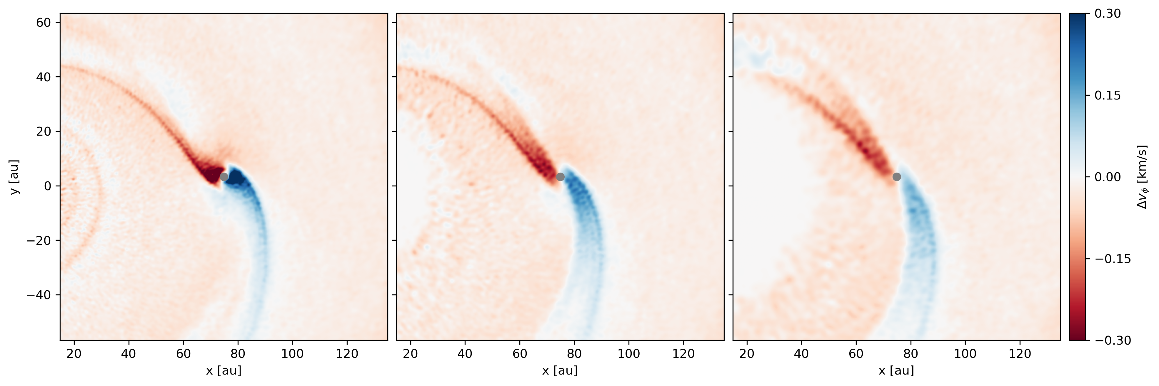
Deviation from Keplerian velocity around a planet: at the disc midplane (left), and 10 (middle) and 20 au (right) above the disc midplane. See here for details.

Analysis

Extra quantities not written to the snapshot file are available:

>>> snap['angular_momentum']
array([ ... ]) <Unit('kilogram * meter ** 2 / second')>

You can generate radial profiles on the snapshot. For example, to calculate the scale height in a disc:

>>> prof = plonk.load_profile(snap)

>>> prof['scale_height']
array([ ... ]) <Unit('meter')>

Physical units of array quantities and other properties allow for unit conversion:

>>> pos = snap['position'][0]
>>> pos
array([-3.69505001e+12,  7.42032967e+12, -7.45096980e+11]) <Unit('meter')>

>>> pos.to('au')
array([-24.6998837 ,  49.60184016,  -4.98066567]) <Unit('astronomical_unit')>

You can get a subset of particles as a SubSnap.

>>> subsnap = snap[:1000]
>>> subsnap = snap[snap['x'] > 0]
>>> subsnap = snap.family('gas')

More

For further usage, see documentation. The code is internally documented with docstrings. Try, for example, help(plonk.Snap) or help(plonk.load_snap).

Install

Conda

You can install Plonk via the package manager Conda from conda-forge.

conda install plonk --channel conda-forge

This will install the required dependencies.

Note: You can simply use conda install plonk if you add the conda-forge channel with conda config --add channels conda-forge. I also recommend strictly using conda-forge which you can do with conda config --set channel_priority true. Both of these commands modify the Conda configuration file ~/.condarc.

pip

You can also install Plonk from PyPI via pip.

python -m pip install plonk

This should install the required dependencies.

Source

You can install Plonk from source as follows.

# clone via HTTPS
git clone https://github.com/dmentipl/plonk.git

# or clone via SSH
git clone [email protected]:dmentipl/plonk

cd plonk
python -m pip install -e .

This assumes you have already installed the dependencies. One way to do this is by setting up a conda environment. The environment.yml file provided sets up a conda environment "plonk" for using or developing Plonk.

conda env create --file environment.yml
conda activate plonk

Requirements

Python 3.6+ with h5py, matplotlib, numba, numpy, pandas, pint, scipy, toml. Installing Plonk with conda or pip will install these dependencies.

Getting help

If you need help, please try the following:

1. Check the documentation.
2. Check the built-in help, e.g. help(plonk.load_snap).
3. Raise an issue, as a bug report or feature request, using the issue tracker.

Please don't be afraid to raise an issue. Even if your issue is not a bug, it's nice to have the question and answer available in a public forum so we can all learn from it together.

If you don't get an immediate response, please be patient. Plonk is maintained by one person, @dmentipl.

Contributing

All types of contributions are welcome from all types of people with different skill levels.

Thank you for considering contributing to Plonk. There are many ways to contribute:

1. If you find any bugs or cannot work out how to do something, please file a bug report in the issue tracker. Even if the issue is not a bug it may be that there is a lack of documentation.
2. If you have any suggestions for new features, please raise a feature request in the issue tracker.
3. If you use Plonk to do anything please consider contributing to the examples section in particular, or any other section, of the documentation.
4. If you would like to contribute code, firstly thank you! We take code contributions via pull request.

See CONTRIBUTING.md for detailed guidelines on how to contribute.

Citation

If you use Plonk in a scientific publication, please cite the paper published in JOSS.

Plonk: Smoothed particle hydrodynamics analysis and visualization with Python

A BibTeX entry is available in CITATION.bib

If you use the interpolation to pixel grid component of Plonk please cite the Splash paper. You should also consider citing any other scientific software packages that you use.

Change log

The change log is available in CHANGELOG.md

plonk's Issues

Change from splash.py to sph-interp

Currently, the low-level SPH interpolation routines live in splash.py. These are rewritten from the original Splash Fortran routines using NumPy and Numba for performance.

The package sph-interp contains very similar functions. Plonk should use this package instead of splash.py. Given that these functions are quite "low-level" it makes sense that they live outside of the Plonk repository. Then other packages can use them.

Add Snap method to set units to physical quantities

Is your feature request related to a problem? Please describe

It would be nice to have a method, say snap.physical_units() that sets the snap to give arrays and other values in physical units rather than having to multiply by the appropriate combination of snap.properties['utime'], snap.properties['udist'], snap.properties['umass'].

Describe the solution you'd like

Implement a method on the snap like snap.physical_units() with arguments to set the time, mass, distance units, such that when accessing arrays like snap['position'] they return an array with physical units.

This solution could return a NumPy array in the correct units. Or, perhaps a better option is to return a Pint array which contains the units along with the array.

Describe alternatives you've considered

The alternative is to continue to do this manually with the units provided in snap.properties.

Additional context

We could use unyt or Astropy units instead.

Add support for more Phantom equations of state

Phantom has integer codes ieos that determine the equation of state (eos). These codes are written to the snapshot file header. These are required to calculate the temperature or pressure as these variables are not written to file. The meaning of the ieos codes can be inferred from the source code eos.F90.

Currently, Plonk supports:

• ieos=1: globally isothermal eos,
• ieos=2: adiabatic eos,
• ieos=3: vertically isothermal eos (appropriate for discs).

We should add support for more Phantom equations of state.

For reference, here is the list of values at the current version:

! This module contains stuff to do with the equation of state
!  Current options:
!     1 = isothermal eos
!     2 = adiabatic/polytropic eos
!     3 = eos for a locally isothermal disc as in Lodato & Pringle (2007)
!     4 = GR isothermal
!     6 = eos for a locally isothermal disc as in Lodato & Pringle (2007),
!         centered on a sink particle
!     7 = z-dependent locally isothermal eos
!     8 = Barotropic eos
!     9 = Piecewise polytrope
!    10 = MESA EoS
!    11 = isothermal eos with zero pressure
!    12 = ideal gas with radiation pressure
!    14 = locally isothermal prescription from Farris et al. (2014) for binary system
!    15 = Helmholtz free energy eos
!    16 = Shen eos
!    19 = Variable gamma (requires KROME)

Add convenience function to generate movies

This could use matplotlib animations, https://matplotlib.org/api/animation_api.html.

Error in Column density plots when using logarithmic colour bar.

Describe the bug

Using the image(quanity='density') method to produce integrated density plots with a logarithmic colour bar causes artefact in regions of a disc where there are no particles. The minimum density colour does not extend to the edges of the box or fill in the gap around the sink

To Reproduce

import plonk
snap = plonk.load_snap('disc_00010.h5')
units = {'position': 'au', 'density': 'g/cm^3', 'projection': 'cm'}
snap.image(
... quantity='density',
... extent=(-120,120,-120,120),
... units=units,
... norm='log',
... vmin=1,
... vmax=3000,
... )
plt.show()

No error is produced, the plot is produced successfully but does not look correct when using the norm='log' option.

Expected behaviour

Expected the plotted area to be filled with the colour corresponding to vmin

Screenshots

Examples

Use the attached .h5 file with plonk (code above) to reproduce problem

Environment

• OS: MacOS Catalina 10.15.7
• Python: Python 3.8.6
• Plonk version: plonk 0.7.3

Data source

disc_00010.h5.zip

Creating arbitrary cross sections through SPH data

Describe the feature request

Implementing the ability to produce slices though the SPH data across any arbitrary plane. Right now Plonk can only do this for the xy-plane, giving slices with constant z. When this is rotated, the slice stays in the xy plane, even the plane of the disc is no longer in the xy plane (but originally was).

Describe the solution you'd like

The ability to be able to produce cross-sectional slices across any arbitrary plane, or possibly even a 3D surface.

e.g. being able to slice across a plane inclined with respect to the xy plane.

More advanced:
Being able to define a 3D surface to, for example, take into account the flaring of a disc, so that we can see how quantities change along a constant disc scale height.

[JOSS review] sample data needed

Is your feature request related to a problem? Please describe

The docs have a getting started section, but in order to play along, we need the sample data. The results of each step should be provided as well so we can verify the library is working as intended.

Describe the solution you'd like

sample dataset referenced in the docs should be included

Describe alternatives you've considered

A clear and concise description of any alternative solutions or features you've considered.

Additional context

Add any other context or screenshots about the feature request here.

TypeError: expected dtype object, got 'numpy.dtype[float64]' when animating

Hi,

I'm trying to visualise my phantom simulation but I keep getting the error TypeError: expected dtype object, got 'numpy.dtype[float64]'

I've tried a few different methods of visualising the sim but the TypeError persists.

Here is a minimum working example using the minor and major phantom dumps.

import plonk
import matplotlib.pyplot as plt

sim = plonk.load_simulation(prefix='disc', directory='hd100453_gas_disc_10mj_20au_low_acc/')

snaps = sim.snaps

units = {'position': 'au', 'density': 'g/cm^3'}

plonk.visualize.animation_images(filename='plots/hd100453_gas_disc_10mj_20au_low_acc.mp4',snaps=snaps,
	units=units,
	quantity='density',
	save_kwargs={'fps': 10, 'dpi': 300},)

This produces the following error.

---------------------------------------------------------------------------
TypeError                                 Traceback (most recent call last)
/Volumes/phd_backup/phantom_dumps/animate_models.py in <module>
     16 'projection': 'cm'
     17 }
---> 18 plonk.animate(
     19 filename='animation.mp4',
     20 snaps=snaps,

/anaconda3/envs/py38/lib/python3.8/site-packages/plonk/visualize/animation.py in animate(filename, snaps, profiles, quantity, x, y, fig, adaptive_colorbar, adaptive_limits, text, text_kwargs, func_animation_kwargs, save_kwargs, **kwargs)
    149             )
    150         else:
--> 151             anim = animation_images(
    152                 filename=filename,
    153                 snaps=snaps,

/anaconda3/envs/py38/lib/python3.8/site-packages/plonk/visualize/animation.py in animation_images(filename, snaps, quantity, fig, adaptive_colorbar, text, text_kwargs, func_animation_kwargs, save_kwargs, **kwargs)
    247 
    248     if fig is None:
--> 249         ax = snaps[0].image(quantity=quantity, **kwargs)
    250         fig = ax.figure
    251         image = ax.images[0]

/anaconda3/envs/py38/lib/python3.8/site-packages/plonk/visualize/visualization.py in image(snap, quantity, x, y, interp, weighted, slice_normal, slice_offset, extent, units, ax, ax_kwargs, colorbar_kwargs, **kwargs)
    145     """
    146     with snap.context(cache=True):
--> 147         return _interpolation_plot(
    148             snap=snap,
    149             quantity=quantity,

/anaconda3/envs/py38/lib/python3.8/site-packages/plonk/visualize/visualization.py in _interpolation_plot(snap, quantity, x, y, kind, interp, weighted, slice_normal, slice_offset, extent, units, ax, ax_kwargs, colorbar_kwargs, **kwargs)
    339     # Interpolate data to plot
    340     num_pixels = _kwargs.pop('num_pixels', None)
--> 341     _data, _extent, _units = _interpolated_data(
    342         snap=snap,
    343         quantity=quantity,

/anaconda3/envs/py38/lib/python3.8/site-packages/plonk/visualize/visualization.py in _interpolated_data(snap, quantity, x, y, interp, weighted, slice_normal, slice_offset, extent, units, num_pixels)
    400 
    401     # Interpolate in code units
--> 402     interpolated_data = interpolate(
    403         snap=snap,
    404         quantity=quantity,

/anaconda3/envs/py38/lib/python3.8/site-packages/plonk/visualize/interpolation.py in interpolate(snap, quantity, x, y, interp, weighted, slice_normal, slice_offset, extent, num_pixels)
    125 
    126     if _quantity.ndim == 1:
--> 127         interpolated_data = scalar_interpolation(
    128             quantity=_quantity,
    129             x_coordinate=x,

/anaconda3/envs/py38/lib/python3.8/site-packages/plonk/visualize/interpolation.py in scalar_interpolation(quantity, x_coordinate, y_coordinate, dist_from_slice, extent, smoothing_length, particle_mass, hfact, weighted, num_pixels)
    208         shape (npixx, npixy).
    209     """
--> 210     return _interpolate(
    211         quantity=quantity,
    212         x_coordinate=x_coordinate,

/anaconda3/envs/py38/lib/python3.8/site-packages/plonk/visualize/interpolation.py in _interpolate(quantity, x_coordinate, y_coordinate, dist_from_slice, extent, smoothing_length, particle_mass, hfact, weighted, num_pixels)
    352         )
    353     else:
--> 354         interpolated_data = interpolate_projection(
    355             x=x_coordinate,
    356             y=y_coordinate,

TypeError: expected dtype object, got 'numpy.dtype[float64]'

• OS: macOS 10.14.6
• Python: Python 3.8.5, Anaconda with conda 4.8
• Plonk version: 0.7.3

I can share the dumps if you need.

Cheers,
Brodie

Plot dust density for one-fluid dump

Describe the bug

I tried different things in order to plot the dust density map in case of a one-fluid dump, without success.

To Reproduce

Steps to reproduce the behaviour:

1. Load data

filename = 'mdisc010racc01_00050.h5' 
snap = plonk.load_snap(filename)

2a. Gas visualisation (works fine):

viz = plonk.visualize.plot( snap=snap,
quantity='density',
extent=(-250, 250, -250, 250),
cmap='gist_heat')

2b. Dust visualisation (doesn't work):

viz = plonk.visualize.plot( snap=snap,
quantity='dust_density',
extent=(-250, 250, -250, 250),
cmap='gist_heat')

3. Since dust_density is in the snap.available_arrays() I was expecting to be able to plot it. Instead, I got this error:

ValueError: 2d quantity must be a vector quantity, e.g. "velocity".
For dust quantities, try appending the dust species number,
e.g. "dust_density_001".

I tried also using dust_density_001, without having success.
I checked and apparently density and dust_density are respectively a line array and a column array. Thinking this could be the problem I converted the dust_density into a "line array", but also this doesn't work.

I also tried defining a new snap quantity:
snap['dust_dens']=snap['density']*snap['dust_fraction']
but it is incredibly slow and my notebook crashes.

Expected behaviour

I would expect to be able to plot the dust density map like the one plotted for the gas, when visualising a one-fluid dump.

Environment:

• OS: e.g. macOS 10.12.6
• Python: Python 3.7, Anaconda with conda 4.7.12, using Jupyter-lab notebook
• Plonk version: 0.5.0

Data source

• SPH code: Phantom, commit version 931253a6f3b49940d2ec4d41e40a95c2e95e2d02, one-fluid method

[JOSS review] Example render usages

The documentation covers loading, and making basic renders, but requires some API exploration to determine how to use render to, for instance, visualize along a different axis.

Having in the docs examples that show rotating the snap, then render-ing the snap, would make this process more obvious.

Shifting to the centre of the disc

Describe the bug

Hi, I'm attempting to shift to the disc centre for both snap images and an animation. In phantom I set a 5mj companion at 10au but the sink position in plonk is significantly far from this.

To Reproduce

I rotate and shift the disc with:

snap_file = 'hd100453_bec_run_5mj_10au/disc_00101.h5'
snap = plonk.load_snap(snap_file)
analysis.discs.rotate_face_on(snap)
com = analysis.total.center_of_mass(snap, sinks=False)
snap.translate(-com)

Then setting the units and printing the sink positions:

snap.set_units(position='au')
print(snap.sinks['position'])

The output.

[[1.0657612036467647 -0.7482025165997441 0.08040807544826903] [151.16832435718015 -17.357874795606797 -215.90554676449221] [-14942.404548791676 35342.100422533564 18413.824209907314]] astronomical_unit

If I print the mass with

print(snap.sinks['mass'])

The output:

[3.3820768744152954e+30 3.9782982217579486e+29 9.490655967300002e+27] kilogram

Therefor the third sink is clearly the 5mj companion but the xyz coordinates are obviously not at a 10au radius.

Is this a plonk issue for a phantom issue?

As for the animation, I'm not sure how to centre the disc at all or label the sinks with a marker. Any tips?
I load the entire simulation with:

sim = plonk.load_simulation(prefix='disc', directory='hd100453_bec_run_5mj_10au/')

Environment (please complete the following information)

• OS: macOS 11.2
• Python 3.8.8
• Plonk version: 0.7.3

Images

It appears that I'm shifting correctly to the star sink.

Data

Here's the phantom disc.setup for reference

# input file for disc setup routine

# resolution
                  np =     1000000    ! number of gas particles

# units
           dist_unit =          au    ! distance unit (e.g. au,pc,kpc,0.1pc)
           mass_unit =      solarm    ! mass unit (e.g. solarm,jupiterm,earthm)

# central object(s)/potential
            icentral =           1    ! use sink particles or external potential (0=potential,1=sinks)
              nsinks =           2    ! number of sinks
             ibinary =           0    ! binary orbit (0=bound,1=unbound [flyby])

# options for binary
                  m1 =       1.700    ! primary mass
                  m2 =       0.200    ! secondary mass
            binary_a =        207.    ! binary semi-major axis
            binary_e =       0.320    ! binary eccentricity
            binary_i =         49.    ! i, inclination (deg)
            binary_O =         47.    ! Omega, PA of ascending node (deg)
            binary_w =         18.    ! w, argument of periapsis (deg)
            binary_f =        180.    ! f, initial true anomaly (deg,180=apastron)
               accr1 =       5.000    ! primary accretion radius
               accr2 =       5.000    ! secondary accretion radius

# options for multiple discs
      use_binarydisc =           F    ! setup circumbinary disc
     use_primarydisc =           T    ! setup circumprimary disc
   use_secondarydisc =           F    ! setup circumsecondary disc
      use_global_iso =           F    ! globally isothermal or Farris et al. (2014)

# options for circumprimary gas disc
      isetgasprimary =           0    ! how to set gas density profile (0=total disc mass,1=mass within annulus,2=surface density normalisation,3=surface density at reference rad\
ius,4=minimum Toomre Q)
    itapergasprimary =           F    ! exponentially taper the outer disc profile
   ismoothgasprimary =           F    ! smooth inner disc
        iwarpprimary =           F    ! warp disc
         R_inprimary =         20.    ! inner radius
        R_refprimary =         20.    ! reference radius
        R_outprimary =         60.    ! outer radius
       disc_mprimary =       0.003    ! disc mass
       pindexprimary =       1.000    ! p index
       qindexprimary =       0.250    ! q index
      posanglprimary =       183.5    ! position angle (deg)
         inclprimary =        14.9    ! inclination (deg)
          H_Rprimary =       0.050    ! H/R at R=R_ref
             alphaSS =       0.005    ! desired alphaSS

# set planets
          setplanets =           1    ! add planets? (0=no,1=yes)
            nplanets =           1    ! number of planets

# planet:1
            mplanet1 =       5.000    ! planet mass (in Jupiter mass)
            rplanet1 =         10.    ! planet distance from star
         inclplanet1 =        14.9    ! planet orbital inclination (deg)
         accrplanet1 =       0.250    ! planet accretion radius (in Hill radius)

# timestepping
             norbits =          10    ! maximum number of outer planet orbits
              deltat =       0.100    ! output interval as fraction of orbital period

Automate building the Conda and pip packages with Travis CI

Automate building the Conda and pip packages with Travis CI.

Issues

Currently, the Conda Forge build recipe requires adding the SHA256 hash from PyPI by hand.

plonk.visualize has no attribute 'render'

I am trying to make a scatter plot of particles by visualize and I get the following error while I follow the instruction of "Plonk tutorial written for the 3rd Phantom + MCFOST users workshop, Monash University, Feb 24-28, 2020". I also used the sample data of the workshop to be sure that data format is not related in problem.

plonk version: 0.7.3
python: 3.7.4
Linux mint 18.1
jupyter lab

import plonk
import matplotlib.pyplot as plt
import numpy as np
filename  = 'path_to_file.h5'
snap = plonk.load_snap(filename)
viz = plonk.visualize.render(snap=snap, quantity='density', extent=[-200, 200, -200, 200])

which raises this error:

---------------------------------------------------------------------------
AttributeError                            Traceback (most recent call last)
<ipython-input-57-c81b5b94f9b3> in <module>
 ----> 1 viz = plonk.visualize.render(snap=snap, quantity='density', extent=[-200, 200, -200, 200])

AttributeError: module 'plonk.visualize' has no attribute 'render'

and when I use dir(plonk.visualize) to return the attributes, render is not in the list.

['__all__',
 '__builtins__',
 '__cached__',
 '__doc__',
 '__file__',
 '__loader__',
 '__name__',
 '__package__',
 '__path__',
 '__spec__',
 'animate',
 'animation',
 'animation_images',
 'animation_particles',
 'animation_profiles',
 'image',
 'interpolate',
 'interpolation',
 'plot',
 'plots',
 'simulation',
 'splash',
 'vector',
 'visualization',
 'visualize_sim']

I also have got an error when using plonk.animate:

FilePath = !ls ./disc_000*.h5
for Filelist in FilePath:
    print(Filelist)
    snaps = plonk.load_snap(Filelist)
    print(snaps)
units = {
        'position': 'au',
        'density': 'g/cm^3',
        'projection': 'cm'
        }
plonk.animate(
        filename='animation.mp4',
        snaps=snaps,
        quantity='density',
        units=units,
        save_kwargs={'fps': 10, 'dpi': 300}
    )    

and after reading and printing all data, this produces the following error.

---------------------------------------------------------------------------
ZeroDivisionError                         Traceback (most recent call last)
<ipython-input-83-349ba0d90912> in <module>
     13         'projection': 'cm'
     14         }
---> 15 plonk.animate(
     16         filename='animation.mp4',
     17         snaps=snaps,

~/anaconda3/envs/plonk-env/lib/python3.8/site-packages/plonk/visualize/animation.py in animate(filename, snaps, profiles, quantity, x, y, fig, adaptive_colorbar, adaptive_limits, text, text_kwargs, func_animation_kwargs, save_kwargs, **kwargs)
    149             )
    150         else:
--> 151             anim = animation_images(
    152                 filename=filename,
    153                 snaps=snaps,

~/anaconda3/envs/plonk-env/lib/python3.8/site-packages/plonk/visualize/animation.py in animation_images(filename, snaps, quantity, fig, adaptive_colorbar, text, text_kwargs, func_animation_kwargs, save_kwargs, **kwargs)
    247 
    248     if fig is None:
--> 249         ax = snaps[0].image(quantity=quantity, **kwargs)
    250         fig = ax.figure
    251         image = ax.images[0]

~/anaconda3/envs/plonk-env/lib/python3.8/site-packages/plonk/visualize/visualization.py in image(snap, quantity, x, y, interp, weighted, slice_normal, slice_offset, extent, units, ax, ax_kwargs, colorbar_kwargs, **kwargs)
    145     """
    146     with snap.context(cache=True):
--> 147         return _interpolation_plot(
    148             snap=snap,
    149             quantity=quantity,

~/anaconda3/envs/plonk-env/lib/python3.8/site-packages/plonk/visualize/visualization.py in _interpolation_plot(snap, quantity, x, y, kind, interp, weighted, slice_normal, slice_offset, extent, units, ax, ax_kwargs, colorbar_kwargs, **kwargs)
    339     # Interpolate data to plot
    340     num_pixels = _kwargs.pop('num_pixels', None)
--> 341     _data, _extent, _units = _interpolated_data(
    342         snap=snap,
    343         quantity=quantity,

~/anaconda3/envs/plonk-env/lib/python3.8/site-packages/plonk/visualize/visualization.py in _interpolated_data(snap, quantity, x, y, interp, weighted, slice_normal, slice_offset, extent, units, num_pixels)
    400 
    401     # Interpolate in code units
--> 402     interpolated_data = interpolate(
    403         snap=snap,
    404         quantity=quantity,

~/anaconda3/envs/plonk-env/lib/python3.8/site-packages/plonk/visualize/interpolation.py in interpolate(snap, quantity, x, y, interp, weighted, slice_normal, slice_offset, extent, num_pixels)
    125 
    126     if _quantity.ndim == 1:
--> 127         interpolated_data = scalar_interpolation(
    128             quantity=_quantity,
    129             x_coordinate=x,

~/anaconda3/envs/plonk-env/lib/python3.8/site-packages/plonk/visualize/interpolation.py in scalar_interpolation(quantity, x_coordinate, y_coordinate, dist_from_slice, extent, smoothing_length, particle_mass, hfact, weighted, num_pixels)
    208         shape (npixx, npixy).
    209     """
--> 210     return _interpolate(
    211         quantity=quantity,
    212         x_coordinate=x_coordinate,

~/anaconda3/envs/plonk-env/lib/python3.8/site-packages/plonk/visualize/interpolation.py in _interpolate(quantity, x_coordinate, y_coordinate, dist_from_slice, extent, smoothing_length, particle_mass, hfact, weighted, num_pixels)
    352         )
    353     else:
--> 354         interpolated_data = interpolate_projection(
    355             x=x_coordinate,
    356             y=y_coordinate,

ZeroDivisionError: division by zero

Split arrays on SubSnap objects return whole array

Describe the bug

Split arrays on SubSnap objects return whole array. I.e. rather than getting only 'x' array you get the whole 'position' array.

To Reproduce

Steps to reproduce the behaviour:

1. Create a SubSnap before accessing any Snap arrays.
2. Access, e.g., 'x' array.
3. Returns whole 'position' array.

import plonk

snap = plonk.load_snap(path_to_snap_file)
subsnap = snap[snap['id'] < 10]
x = subsnap['x']
x.shape
# prints (n_particles, 3)

Expected behaviour

subsnap['x'] should just return the 'x' array.

Environment

• macOS 10.15.1
• Python 3.7
• Plonk version 0.2.1

Animation is broken

Describe the bug

The plonk.animation function no longer works.

To Reproduce

import plonk
sim = plonk.load_sim('disc')
plonk.animation(
    filename='density.mp4',
    snaps=sim.snaps,
    quantity='density',
)

This produces the following error.

---------------------------------------------------------------------------
TypingError                               Traceback (most recent call last)
<ipython-input-3-d7a778b00f2e> in <module>
----> 1 plonk.animation(
      2     filename='density.mp4',
      3     snaps=sim.snaps,
      4     quantity='density',
      5 )

~/repos/plonk/plonk/visualize/animation.py in animation(filename, snaps, quantity, x, y, extent, fig, adaptive_colorbar, text, text_kwargs, func_animation_kwargs, save_kwargs, **kwargs)
    204         fig, animate, frames=len(snaps), **func_animation_kwargs
    205     )
--> 206     anim.save(filepath, extra_args=['-vcodec', 'libx264'], **save_kwargs)
    207     plt.close()
    208     if tqdm is not None:

~/conda/lib/python3.8/site-packages/matplotlib/animation.py in save(self, filename, writer, fps, dpi, codec, bitrate, extra_args, metadata, extra_anim, savefig_kwargs, progress_callback)
   1118                                _is_saving=True, manager=None):
   1119             for anim in all_anim:
-> 1120                 anim._init_draw()  # Clear the initial frame
   1121             frame_number = 0
   1122             # TODO: Currently only FuncAnimation has a save_count

~/conda/lib/python3.8/site-packages/matplotlib/animation.py in _init_draw(self)
   1693         # artists.
   1694         if self._init_func is None:
-> 1695             self._draw_frame(next(self.new_frame_seq()))
   1696
   1697         else:

~/conda/lib/python3.8/site-packages/matplotlib/animation.py in _draw_frame(self, framedata)
   1716         # Call the func with framedata and args. If blitting is desired,
   1717         # func needs to return a sequence of any artists that were modified.
-> 1718         self._drawn_artists = self._func(framedata, *self._args)
   1719         if self._blit:
   1720             if self._drawn_artists is None:

~/repos/plonk/plonk/visualize/animation.py in animate(idx)
    179             else:
    180                 _extent = extent
--> 181             interp_data = interpolate(
    182                 snap=snaps[idx],
    183                 interp=interp,

~/repos/plonk/plonk/visualize/interpolation.py in interpolate(snap, quantity, x, y, interp, z_slice, extent, **kwargs)
     91
     92     if _quantity.ndim == 1:
---> 93         interpolated_data = scalar_interpolation(
     94             quantity=_quantity,
     95             x_coordinate=x,

~/repos/plonk/plonk/visualize/interpolation.py in scalar_interpolation(quantity, x_coordinate, y_coordinate, z_coordinate, extent, smoothing_length, particle_mass, hfact, number_of_pixels, cross_section, density_weighted)
    175         shape (npixx, npixy).
    176     """
--> 177     return _interpolate(
    178         quantity=quantity,
    179         x_coordinate=x_coordinate,

~/repos/plonk/plonk/visualize/interpolation.py in _interpolate(quantity, x_coordinate, y_coordinate, z_coordinate, extent, smoothing_length, particle_mass, hfact, number_of_pixels, cross_section, density_weighted)
    331         )
    332     else:
--> 333         interpolated_data = interpolate_projection(
    334             x=x_coordinate,
    335             y=y_coordinate,

~/conda/lib/python3.8/site-packages/numba/core/dispatcher.py in _compile_for_args(self, *args, **kws)
    413                 e.patch_message(msg)
    414
--> 415             error_rewrite(e, 'typing')
    416         except errors.UnsupportedError as e:
    417             # Something unsupported is present in the user code, add help info

~/conda/lib/python3.8/site-packages/numba/core/dispatcher.py in error_rewrite(e, issue_type)
    356                 raise e
    357             else:
--> 358                 reraise(type(e), e, None)
    359
    360         argtypes = []

~/conda/lib/python3.8/site-packages/numba/core/utils.py in reraise(tp, value, tb)
     78         value = tp()
     79     if value.__traceback__ is not tb:
---> 80         raise value.with_traceback(tb)
     81     raise value
     82

TypingError: Failed in nopython mode pipeline (step: nopython frontend)
non-precise type pyobject
During: typing of argument at /Users/daniel/repos/plonk/plonk/visualize/splash.py (157)

File "../../../repos/plonk/plonk/visualize/splash.py", line 157:
def interpolate_projection(
    <source elided>
    """
    coltable = setup_integratedkernel()
    ^

This error may have been caused by the following argument(s):
- argument 7: cannot determine Numba type of <class 'pint.quantity.build_quantity_class.<locals>.Quantity'>
- argument 8: cannot determine Numba type of <class 'pint.quantity.build_quantity_class.<locals>.Quantity'>
- argument 11: cannot determine Numba type of <class 'pint.quantity.build_quantity_class.<locals>.Quantity'>
- argument 12: cannot determine Numba type of <class 'pint.quantity.build_quantity_class.<locals>.Quantity'>

Expected behaviour

I expect it to produce a file "density.mp4" with an animation of the rendered density.

Environment (please complete the following information)

• OS: macOS 10.15.6
• Python: Python 3.8
• Plonk version: 0.6.0

Data source

I used the dataset from the documentation (https://anaconda.org/dmentipl/plonk_example_data/).

Additional context (optional)

I think the issue is in returning non-dimensional data, and needing to add units.

            interp_data = interpolate(
                snap=snaps[idx],
                interp=interp,
                quantity=quantity,
                x=x,
                y=y,
                extent=_extent,
                **_kwargs,
            )

Use Dask for lazy loading and delayed operations

Accessing a particle array on a snapshot is currently lazy, in the sense that the data is only loaded from disc into memory when requested, e.g. with snap['position']. However, it remains there in the dictionary snap._arrays.

An alternative is to load the array as a Dask array and use the resulting object as if it were a NumPy array loaded into memory. Then complicated expressions can be written before anything is loaded into memory. The computation is executed with the .compute() method. Dask also allows for easy parallelization on both local, i.e. a multi-core laptop, and remote hardware, i.e. a supercomputing cluster.

A suggestion is to adjust the __getitem__() method to return a Dask array, and to not store the array in snap._arrays.

Add function to modify snaps and write a new one

Is your feature request related to a problem? Please describe

This function is to replicate the functionality of Phantom's moddump.

Describe the solution you'd like

A new module/class/function to modify snapshots and write new ones to file.

Only the first profile in list is plotted

I am using Plonk to make a profile plot and I have a problem with that. After reading the list of profiles and appending them, only the first snap is plotted.

plonk version: 0.7.3
python: 3.7.4
Linux mint 18.1
jupyter lab

import plonk
import matplotlib.pyplot as plt
import numpy as np

filename = 'file_address'
snap = plonk.load_snap(filename)

snap = plonk.load_snap(filename)
snap.add_quantities('disc')
prof = plonk.load_profile(snap, cmin='10 au', cmax='200 au')

snap['timestep'].to('Myr')

snap['x'].to('pc')

sim = plonk.load_simulation(prefix='disc')

sinkFilePath = !ls 'my sink_file_path'

times = sim.properties['time'].to('Myr')

for sinklist in sinkFilePath:
    print(sinklist)
    profiles = list()
    snap = plonk.load_snap(sinklist)
    profile = plonk.load_profile(snap, cmin='10 au', cmax='150 au', n_bins=50)
    profiles.append(profile)

fig, ax = plt.subplots()
units = {'position': 'pc', 'density': 'g/cm^3'}
for time, profile in zip(times, profiles):
    label = f'{time.m:.0f}'
    profile.plot(
        'radius', 'density', units=units, label=label, ax=ax
    )
ax.set_ylabel('Density [g/cm${}^3$]')
ax.legend(title='Time [Myr]', loc='best')

I also need to plot multiple snapshots in a single panel. I used to do it with splash and I want to know if it is possible in plonk. I expect a plot similar to what splash produces.
multiple_plot.pdf

Tracking individual particles

Hi Daniel,

I hope you are well. I'm trying to track individual particles from snapshot to snapshot through the simulation and am having some issues. I thought of using the particle ID numbers but these don't seem to be allocated to the same particles in one snapshot as they are in the next.
Is there something I am missing that enables the user to do something like this? Find the ID number of a particle at x1,y1,z1 at t = t_1 and then, using that ID number, find x2,y2,z2 of the particle at t = t2?

Colorbar not displayed properly in the Multiplot class

Describe the bug

When using the visualization.MultiPlot class, the colorbars are not displayed properly. There are two issues.

1. When using 'render_scale': 'log', the image is rendered correctly, but the colorbar remains linear.
2. When choosing a shape different from (1 x N) or (N x 1), the colorbars of some subplots are not displayed at all.

I am plotting a Phantom dump obtained with a one fluid multigrain simulation.
This is part of the code I'm using for the multiplot:

totdustfrac = np.zeros(1000000)

for s in range(0,5):
    grains = dump.header['grainsize'][s]*dump.header['udist']*10**(4) 
    dustfrac = dump.particles.arrays['dustfrac'][:,s]
    totdustfrac +=dump.particles.arrays['dustfrac'][:,s]

new_units = plonk.Units(length='au', mass='g', time='yr', density=1., velocity=1.0e5)
density = dump.density
density = dump.units.convert_quantity_to_new_units(density, 'density', new_units)

gas_density = density*(1.-totdustfrac)

options = list()
options.append({'render': gas_density,
                'render_scale': 'log',
                'extent': [-100,100,-100,100],
                'inclination': -65,
                'position_angle': -21,
                'normalize':False,
                'render_label': r'$\Sigma_{\rm gas}$ [g cm${}^{-2}$]',
                'integrated_z':plonk.constants.au,
               })

label_dust = [r'$\Sigma_{{\rm d},1.77\,\mu{\rm m}}$ [g cm${}^{-2}$]',
              r'$\Sigma_{{\rm d},5.56\,\mu{\rm m}}$ [g cm${}^{-2}$]',
              r'$\Sigma_{{\rm d},0.017\,{\rm mm}}$ [g cm${}^{-2}$]',
              r'$\Sigma_{{\rm d},0.054\,{\rm mm}}$ [g cm${}^{-2}$]',
              r'$\Sigma_{{\rm d},0.17\,{\rm mm}}$ [g cm${}^{-2}$]',
              r'$\Sigma_{{\rm d},0.54\,{\rm mm}}$ [g cm${}^{-2}$]',
              r'$\Sigma_{{\rm d},1.7 {\rm mm}}$ [g cm${}^{-2}$]']
    
    
for s in range(0,5):
    options.append({'render': density*dump.particles.arrays['dustfrac'][:,s],
                   'render_scale': 'log',
                   'extent': [-100,100,-100,100],
                   'inclination': -65,
                   'position_angle': -21,
                   'render_label': label_dust[s],
                   'font_size': 30, 
                    'normalize': False,
                    'integrated_z':plonk.constants.au,
                   })

    

multiplot = plonk.visualization.MultiPlot(
    dump,
    options,
    scale=7,
    shape=(3,2),
    axes_pad=0.7,
    cbar_mode='each',
    cbar_location='top',
    cbar_pad=0.2
)

Expected behavior

NxM subplots, each with a colorbar in log scale.

Screenshots

Here you can see the (1x6) shape image, displaying all the colorbars, but not in log scale (the color rendering is performed properly in log). The (6x1) shape is behaving at the same way.

Here you can see the (2x3) shape image, not displaying properly the last colorbars. The colorbar is plotted only for the 0, the 3rd, 4th and 5th element.

Here you can see the (3x2) shape image, not displaying properly the last colorbars. The colorbar is plotted only for the 0, the 2nd, 4th and 5th element.

Environment:

• OS: macOS 10.12.6
• Python :
  - conda version : 4.7.11
  - conda-build version : 3.17.8
  - python version : 3.7.3.final.0
  (using Jupiter-lab)
• Plonk version: 0.1.0

Data source

• SPH code:
  - Phantom,
  - version -> Commit tag: ok-20190328-44-g931253a
  Full commit ID: 931253a6f3b49940d2ec4d41e40a95c2e95e2d02
  - simulation performed with one fluid, multigrain setup.

Sink particles are not rotated with `snap.rotate`

Describe the bug

Sink particles are not rotated with snap.rotate

To Reproduce

Steps to reproduce the behaviour:

import plonk
from scipy.spatial.transform.rotation import Rotation

snap = plonk.load_snap(path_to_file)
rotation = Rotation.from_rotvec([1, 1, 0])

print(snap.sinks['position'])
snap.rotate(rotation)
print(snap.sinks['position'])

The two print statements are the same but should show that the snapshot has been rotated.

Expected behaviour

The sinks should rotate with a snap rotation.

Environment (please complete the following information):

• OS: macOS
• Python: 3.7
• Plonk version: 0.3.0

Data source

• SPH code: Phantom

eccentricity function in profile.py

Describe the bug

In line 329 of profile.py, the definition of velocity reads:
vel = self.Snap['vxyz'][self._mask]
and it should be
vel = self.snap['vxyz'][self._mask]

To Reproduce

after loading a snapshot, running the following code results in an error

prof = plonk.analysis.Profile(snap, radius_min=0, radius_max=6)
ecc = prof._profile_functions["eccentricity"](prof, gravitational_parameter = 2)

Expected behaviour

return radial profile of eccentricity

Environment (please complete the following information):

• OS: [macOS 10.14.6]
• Python: [Python 3.7.3, Anaconda with conda 4.7.12, using Jupyter notebook]
• Plonk version: [0.3.0]

Density plots appear unexpectedly fuzzy

Column density plots in plonk don't appear to show the same information as in splash? I plotted a broken disc and it looked fuzzier than I thought it should and despite adjustments it didn't improve. Have I missed something? It appears that high density structure in the inner region and the gap between the inner and outer disc are not accurately reproduced in plonk? See the examples attached below.

density_plonk.pdf
density_splash.pdf

Following the example in the wiki as much as possible, I plotted with:
viz = plonk.visualize.render(snap=snap,
quantity='density',
axis=axes,
extent=[-15,15,-15,15],
scalar_options={'cmap': 'gist_heat',
'norm': 'log',
'plot_colorbar': cbar}
)

I'm using:

• OS: macOS 10.13.6
• Python: Python 3.7.3, Anaconda with conda 4.7.12, using Jupyter notebook
• Plonk version: 0.2.1
• SPH code: Phantom, version c816ba88, gas only simulation.

Read more Phantom header quantities

Currently the only Phantom header quantities read in are 'time', 'udist', 'utime', 'umass', 'hfact', 'ieos', 'gamma', 'polyk', 'qfacdisc'.

Other quantities may be required.

Should the 'id' array be 'particle_type'?

Should the 'id' array be 'particle_type'? Then 'id' could be an integer that uniquely identifies a particle. This could be useful to track particles through simulations.

Incorrect temperature with phantom models with ieos=2

Describe the bug

Plonk does not appear to to recover the temperature correctly when used on mcfost+phantom dump, indicating temperatures of a few 1e6K for a protoplanetary disc.

To Reproduce

See the data in the dropbox link below, and the following script

"""Calculate vertical profile in discs."""

import matplotlib.pyplot as plt
import numpy as np
import plonk


def vertical_profile(snap, radius, vertical_height, radial_width=1):
    """Vertical profile at particular radius.

    Parameters
    ----------
    snap
        The Snap.
    radius
        The radius at which to calculate the vertical profile.
    vertical_height
        The height over which to compute the vertical profile.
    radial_width
        The radial width of the subset of particle on which to compute
        the vertical profile.
    """
    # Load extra quantities, e.g. cylindrical radius
    snap.extra_quantities()

    # Generate subsnap in a cylindrical ring
    subsnap = snap[
        (snap['R'] > radius - radial_width / 2)
        & (snap['R'] < radius + radial_width / 2)
    ]

    # Return Cartesian z-profile
    return plonk.load_profile(
        subsnap,
        ndim=1,
        coordinate='z',
        radius_min=-vertical_height / 2,
        radius_max=vertical_height / 2,
    )


if __name__ == '__main__':

    # Load snapshot
    snap = plonk.load_snap('hydrostatic_18790.h5')

    # Set molecular weight for temperature
    snap.set_molecular_weight(2.381)

    # Choose radii at which to calculate z-profiles.
    radius = np.linspace(25, 150, 5)

    # Vertical height
    R0 = 10  # reference radius
    H0 = 0.034 * R0  # scale height at reference
    q = 1 / 4  # sound speed index
    scale_height = H0 * (radius / R0) ** (3 / 2 - q)
    vertical_height = 10 * scale_height

    # Make figure and axes
    fig, axs = plt.subplots(ncols=2, figsize=(12, 5))
    axs[0].set(xlabel='altitude', ylabel='density')
    axs[1].set(xlabel='altitude', ylabel='temperature')

    # Loop over all radii and plot density and temperature profiles
    for R, dZ in zip(radius, vertical_height):
        prof = vertical_profile(snap=snap, radius=R, vertical_height=dZ)
        prof.plot('radius', 'density', label=f'radius={R:.0f}', ax=axs[0])
        prof.plot('radius', 'temperature', label=f'radius={R:.0f}', ax=axs[1])

    axs[1].legend().remove()
    plt.show()

Expected behaviour

I would love to get the correct mcfost temperature ;-)

Screenshots

Environment (please complete the following information):

• OS: MacOS 10.15.6
• Python: python 3.7 (conda)
• Plonk version: 0.5.3

Data source

https://www.dropbox.com/sh/goc9rukjghnca0d/AAABP1n5N-iRlAukFkwUAAmda?dl=0

plonk.visualize.plot passes colorbar_kwargs to imshow

I am trying to change the position of the colorbar to the left hand side of the plot. I think I should be able to do this by setting colorbar_kwargs={'position': 'left'}, but this raises the error
AttributeError: 'AxesImage' object has no property 'colorbar_kawrgs'

It seems that colorbar_kwargs is getting passed to the plots.imshow function, which raises this error.

The code below reproduces the error

dumpfile = 'internal/e40_q2_gtd/rescale_hires_00092.h5'

snap= plonk.load_snap(dumpfile)

RENDER = 'density'

dens = plonk.visualize.plot(snap=snap, quantity=RENDER,
                     show_colorbar=True, cmap='gist_heat', norm='log', colorbar_kwargs={'position': 'left'})

Also another thing I noticed in the documentation for plonk.visualize.plot, it states it returns a matplotlib axes object:

    Returns
    -------
    ax
        The matplotlib Axes object.

However, this does not seem to be the case:

>>> print(dens)
<plonk.Visualization "rescale_hires_00092.h5">

I am also wondering if it is possible to make the plot_object object available to the user somehow in the above object, or make it accessible some other way. It would be useful if one wants to have more control over other matplotlib features themselves. For example, if I wanted to customise the colorbar after making the plot, I need plot_object to do so.

Add other snapshot formats

Would you be interested in adding support for other snapshot formats, e.g. the AMUSE HDF5 format?

access to setup and in file

I need access to some properties of the simulation itself (number of particles, accretion radius of the sinks, alpha_av etc).
For now, I just did a small function in order to extract this data and have it in a dictionary, but I think it would be useful to have it inside the simulation class, or just have a plonk function to take the .setup and .in file and load them.