climatemargo / climatemargo.jl

Julia implementation of MARGO, an idealized climate-economic modelling framework for Optimizing trade-offs between emissions Mitigation, Adaptation, carbon dioxide Removal, and solar Geoengineering.

ClimateMARGO.jl

A Julia implementation of MARGO, an idealized framework for optimization of climate control strategies.

The MARGO model is described in full in an accompanying Research Article, published Open-Access in the journal Environmental Research Letters. The julia scripts and jupyter notebooks that contain all of the paper's analysis are available in the MARGO-paper repository (these are useful as advanced applications of MARGO to complement the minimal examples included in the documentation).

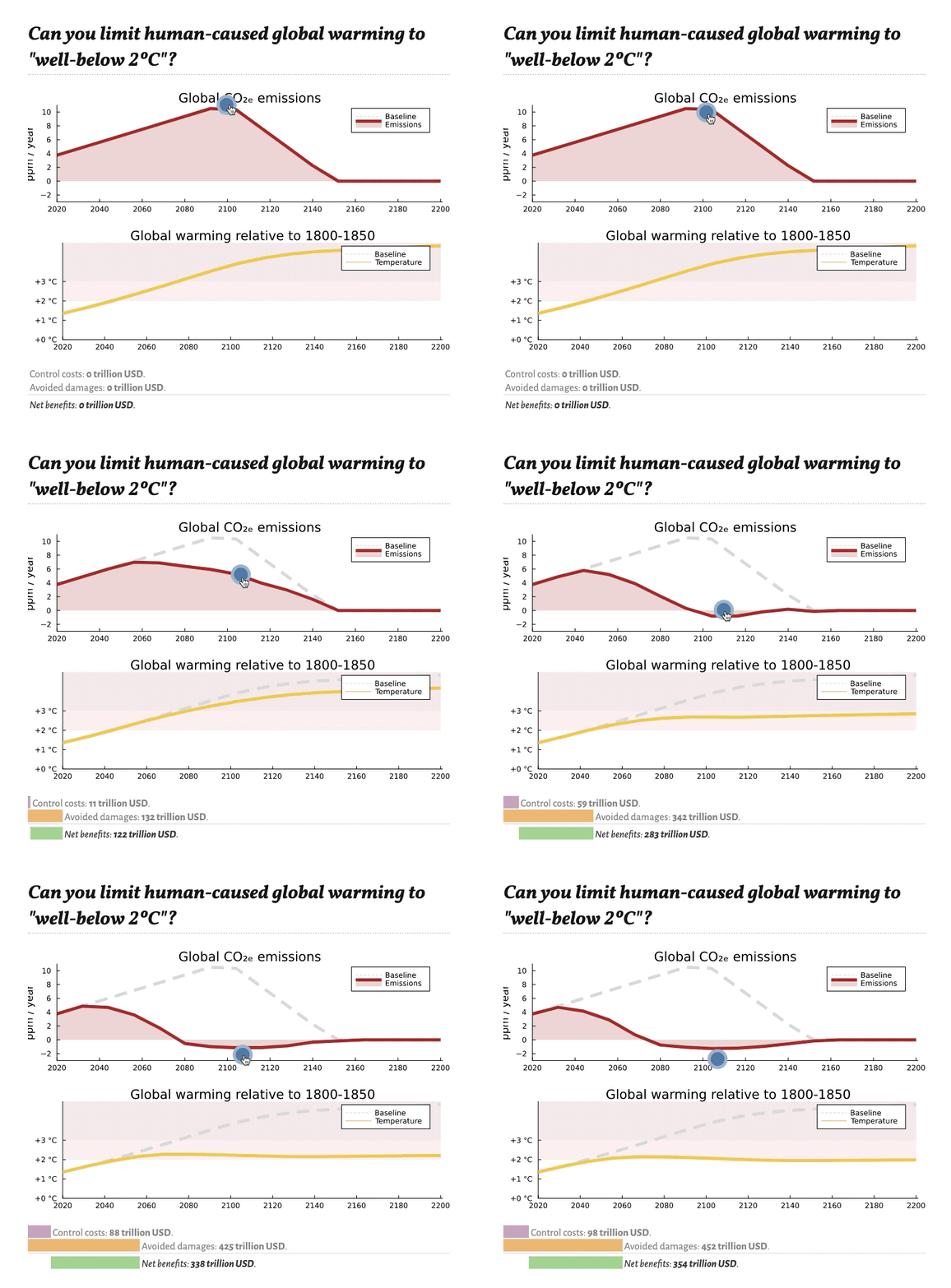
Try out the MARGO model by running our Pluto-based web-app directly in your browser!

ClimateMARGO.jl is currently in beta testing; basic model documentation is slowly being added. Substantial structural changes may still take place before the first stable release v1.0.0. Anyone interested in helping develop the model post an Issue here or contact the lead developer Henri Drake directly (henrifdrake at gmail.com), until explicit guidelines for contributing to the model are posted at a later date.

---

README.md formatting inspired by Oceananigans.jl

climatemargo.jl's Issues

Towards a generic MARGO model structure (with abstract submodel types)

I've been working on implementing a more accurate version of MARGO's 1.5-layer (or "Deep-layer") Energy Balance Model. The improved solution is an exact analytical solution to the two-layer problem (see #43).

I quickly ran into a problem that the MARGO code, as it is currently written, is not nearly as flexible as we would like it to be. In particular, we do not have the appropriate abstractions for allowing submodules to be swapped out for others on the fly.

I imagine that in addition to the bare-bones MARGO configuration, other configurations could be easily created by picking and choosing the complexity of various components. If we define the abstract types in this way, it would also be easier for others in the community to make their own changes and possibly contribute them to the master branch.

One huge advantage of abstract types is that some methods will apply to the abstract types while others will apply to specific model types.

What new feature or storyline would you like to see?

Launching an interactive web-app

Continuing from hdrake/OptimizeClimate#18

Cleanup data structures

Before tackling documentation #2 and unit tests #3, the first priority is to cleanup the data structures (see branch https://github.com/hdrake/ClimateMARGO.jl/tree/data-structure-cleanup).

There are a few features which are particularly undesirable about the current data structures:

1. We hardly use any functions in the JuMP optimization code src/optimization/jl, instead choosing to write out the objective function in its entirety, which is excessively long and susceptible to bugs. My guess is that it is possible to write the objective condition in one line that looks something like (in pseudo-JuMP syntax)

for i in N; @constraint{ T(M,R,G,A) < Tstar }; end

where M, R, G, A are the control variables.
2. The few functions that are currently used in the JuMP optimization code have explicitly re-defined within the optimization code, probably for legacy reasons. Ideally, the diagnostic functions used for plotting / analysis should be re-used for the optimization to reduce the likelihood of discrepancies between the two versions of the code (which indeed caused breaking bugs in early versions of the implementation).
3. There are a lot of redundant functions that should be collapsed into a single function with keyword arguments and/or different methods.
4. We should rethink the ClimateModel, Physics, Controls, and Economics structs. They are fairly unwieldy because I did not really understand Julia constructors when I created them half a year ago. It might be useful to look at how more mature julia models like https://github.com/CliMA/Oceananigans.jl or https://github.com/CliMA/ClimateMachine.jl structure their submodules for inspiration.

Experiment with converting to NLopt instead of JuMP

Right now, margo's optimization is done using JuMP, but we want to use NLOpt.jl instead. The two reasons are:

• Currently, the model has to be written twice in the source code of ClimateMARGO.jl: once in Julia functions, and once in the JuMP syntax. We tried calling the Julia functions from JuMP to avoid this problem, but the performance impact of connecting the two is too large: #18
• JuMP will find a local optimum, but we want a global optimum. We suspect that the current local optima are global, but for different parameter values, this might not be the case. NLOpt.jl can do global optimization. (@hdrake can say more)

Coherent & concise JuMPification of MARGO?

As mentioned in #14, it would be nice to reduce the JuMP implementation of MARGO to a few single-line statements like:

for i in N; @constraint{ T(M,R,G,A) < Tstar }; end
@NLobjective( model_optimizer, Min, net_present_cost(M,R,G,A) );

which reuse the diagnostic functions such as T which fully describe the model (see https://github.com/hdrake/ClimateMARGO.jl/tree/updating-structure) but are complicated functions of both the four controls {M,R,G,A} as well as a number of prescribed inputs functions and parameters. In the current implementation af16f49, these optimization constraints are hard-coded from scratch, span many lines, and are repeated several times over.

Include example of the "policy response process" described in paper

Based on @danielkoll's feedback, I realized the policy response process is only described in MARGO paper (and corresponding notebooks), not anywhere in the existing documentation or examples. We should include a minimal example of the implementation, e.g. what if decision-makers only start considering carbon dioxide removal in 2050?

Just setting

delay_deployment = Dict(
"mitigate"=>0,
"remove"=>30,
"geoeng"=>0,
"adapt"=>0
)

doesn't quite do this because the policy makers in 2020 have perfect knowledge that CDR will become available in 2050 and will include that information in their decision making.

Implement exact solution to two-box energy balance model

Currently, we implement an approximate solution to the two-box energy balance model, which is really more of a 1.5 box solution which assumes the upper-box equilibrates instantly with the forcing. I did this because I did not know how to solve the full two-box equations but thankfully Geoffroy et al. 2013 did this for us and the solution is just a sum of exponential green's functions.

Replace "tutorial.ipynb" with a Literate.jl script

The tutorial notebook is unfortunately out of date and a pain to keep up to date in the current workflow.

I'd like to instead make this a literate script, which will be automatically converted into a markdown file for the documentation website (+ a julia notebook for the binder?) using Literate.jl and Documenter.jl.

Inconsistent naming "M" and "mitigate", nested and flat, struct and Dict

The package has lots of concepts that are 'per technology': M,R,G,A, but their syntax is inconsistent:

Naming

Sometimes we have M, R, G, A,
sometimes mitigate, remove, geoeng (abbreviated), adapt

Nested and flat

Sometimes we have nested properties:
climate_model.controls containing climate_model.controls.M, climate_model.controls.R, etc.,

and sometimes it is a flat structure:
climate_model.economics.mitigate_cost, climate_model.economics.remove_cost, etc.

Struct and Dict

For nested structures, sometimes we use a struct:
climate_model.controls.M

and sometimes we use a Dict:
optimize_controls!(m; max_slope=Dict("mitigate" => ...)

Add optimization constraints as a submodel in ClimateModel or ClimateModelParameters?

Would it be better to include the optimization parameters / constraints as a submodel in ClimateModel or ClimateModelParameters or should they remain as arguments in the optimize_controls! function?

Multiple equilibria

I came up with a simple example of multiple equilibria, which could be used to test the limits of optimization schemes (cc @danielkoll). All I had to do was decrease the exponent of the control costs (here for geoengineering and mitigation) to below p=1, which can be thought of as a crude parameterization for "economies of scale" or "learning rates". This is because marginal costs scale like p-1 and thus decrease with more deployment and so it makes more sense to put all of your eggs in one basket. In this example I tuned the parameters so that it happens that the two local minima are roughly similar, so that there are two roughly equivalent policy options.

Here is a minimal example to reproduce the plot.

# # A simple two-dimensional optimization problem

# ## Loading ClimateMARGO.jl
using ClimateMARGO # Julia implementation of the MARGO model
using PyPlot # A basic plotting package

# Loading submodules for convenience
using ClimateMARGO.Models
using ClimateMARGO.Utils
using ClimateMARGO.Diagnostics

# ## Loading the default MARGO configuration
params = deepcopy(ClimateMARGO.IO.included_configurations["default"])

# Modify parameters to make geoengeering and mitigation costs similar
params.economics.geoeng_cost *= 0.1;
params.economics.mitigate_cost *= 5;

# ### Instanciating the `ClimateModel`
m = ClimateModel(params)

# ## Brute-force parameter sweep method to map out objective function

# ### Parameter sweep
Ms = 0.:0.005:1.0;
Gs = 0.:0.005:1.0;

net_benefit = zeros(length(Gs), length(Ms)) .+ 0.; #

for (o, option) = enumerate(["adaptive_temp", "net_benefit"])
    for (i, M) = enumerate(Ms)
        for (j, G) = enumerate(Gs)
            m.controls.mitigate[t(m) .<= 2100] = zeros(size(t(m)))[t(m) .<= 2100] .+ M
            m.controls.geoeng[t(m) .>= 2150] = zeros(size(t(m)))[t(m) .>= 2150] .+ G
            ### KEY CHANGE: Significantly decrease exponent of both control costs, so that costs are now concave rather than convex functions
            net_benefit[j, i] = net_present_benefit(m, discounting=true, p=0.75, M=true, G=true)
        end
    end
end

# ### Visualizing the two-dimensional optimization problem

fig = figure(figsize=(8, 6))

subplot()
q = pcolor(Ms, Gs, net_benefit, cmap="Greys_r")
cbar = colorbar(label="Net present benefits, relative to baseline [trillion USD]", extend="both")
contour(Ms, Gs, net_benefit, colors="k", levels=20, linewidths=0.5, alpha=0.4)
grid(true, color="k", alpha=0.25)

xlabel("Emissions mitigation level [% reduction]")
xticks(0.:0.2:1.0, ["0%", "20%", "40%", "60%", "80%", "100%"])
ylabel("Geoengineering rate [% of RCP8.5]")
yticks(0.:0.2:1.0, ["0%", "20%", "40%", "60%", "80%", "100%"])
title("Cost-benefit analysis")
gcf()

Inconsistency about whether `t.==present_year` should be included in `future_mask`.

Thanks to @freeman-lab for pointing this out!

Unit tests

I should at least have some unit tests for the key functions.

Model documentation

Should add documentation using Documenter.jl which is mostly made up of documentation markdown files but also also nicely publishes the source code w/ source code docstrings.

Replace PyPlot calls with Plots.jl

@fonsp has mentioned that having PyPlot as a dependency for ClimateMARGO.jl unecessarily complicates things.

I see three options for moving forward:

1. Re-implement plotting functions using Plots.jl
2. Remove plotting submodule from ClimateMARGO.jl and include it in separate PlotMARGO.jl package, or more general utility package
3. Same as (2) but re-implement using Plots.jl

What do you think @fonsp? My understanding is that you already have a hacky way of removing the plotting package dependencies– is this even necessary? I think it might be desirable even for your average user because it will decrease build / binder spin-up time?

"How do I extract ClimateMARGO.jl data as a csv file?"

There are two ways of extracting data from the ClimateModel type. If the data you want is already an argument within the type (or a subtype), then you can just extract it like this:
m.economics.baseline_emissions
If the data does not live within the ClimateModel type (e.g. diagnostics like temperature or CO2 concentrations), then you need to use a diagnostic function that computes those timeseries based on the information in the ClimateModel type. Many of these are included in the Diagnostics submodule. For example, to extract the temperature resulting from mitigated emissions:
temperature = T(m, M=true)

Here is a minimal example of using extracting data to make a csv file (see also the attached csv file that it creates). 

# First, we create an example instance of ClimateMARGO.jl, from which we want to extract some outputs
using ClimateMARGO
using ClimateMARGO.Models
params = deepcopy(ClimateMARGO.IO.included_configurations["default"]);
m = ClimateModel(params);

# Next, we use DataFrames.jl to store time-series of ClimateMARGO.jl diagnostics
# (which the typeof function tells us are of type Array{Float64,1}) as columns.
# We include the "year" as the first column, for reference.
using DataFrames
df = DataFrame(
    year = t(m),
    baseline_emissions = m.economics.baseline_emissions, # or emissions(m, M=false)
    controlled_emissions = emissions(m, M=true)
    temperature = T(m, M=true)
)

# Finally, we use CSV.jl to output this dataframe as a CSV
using CSV
CSV.write("ClimateMARGO_temperature_example.csv", df)

You can see the source code for all of the different diagnostics here: https://github.com/ClimateMARGO/ClimateMARGO.jl/tree/master/src/DiagnosticsIf there is a diagnostic that you are interested in, but that is not yet computed, then you can use the existing diagnostics as a template.

Consistent and correct methods for changing the timestep on the fly.

Quoting @fonsp

I was looking at the new IO functions, I really like the feature of sharing your configuration!

However, I found that the new Economics struct contain baseline_emissions and extra_CO2, which are time series, so they depend on the Domain. This means that:

1. Domain and Economics are not independent parts of ClimateModelParameters
2. You can't modify the domain, in particular when using the default model parameters. Playing around with dt is a way to find out if the discretization affects the result, but that is no longer easy to do.

This also means that the MargoAPI can only use dt=5, but I found that dt=20 has representative results with better performance.

Some ideas:

Storing a time series:

• If we store these as time series, then Domain should be an immutable struct, because changing it will either error, or lead to invisibly false results.
• Store a time series with dt=1, and interpolate into different domains. This might be the easiest solution!

Alternatives to storing a time series:

• Store the parameters describing these series, so for baseline_emissions, that would be the parameters for ramp_emissions.
  (I'm not sure what the plans are for extra_CO2)
  but this would limit what you can use for these parameters

• Store the function itself. So:
  mutable struct Economics
  ...

  baseline_emissions::Function
  extra_CO₂::Function
  end

The problem now is that JSON2 can't convert Functions. So instead, you could store the string:
mutable struct Economics
...

baseline_emissions_code::String
extra_CO₂_code::String

end

and use eval(Meta.parse(code)) to get a Julia function from the code. But this is obviously quite messy.

Let me know what you think!

For the API, I will just reconstruct these two timeseries from a different dt :)

Problems with T_adapt and optimization in 0.2.0

In the code below, I create a model with the default parameters and optimize for the 3C goal, but the result is a 0.8C policy, according to T_adapt, and a 1.6C policy according to T:

julia> import ClimateMARGO

julia> using ClimateMARGO.Models

julia> using ClimateMARGO.Optimization

julia> using ClimateMARGO.Diagnostics

julia> model_parameters = deepcopy(ClimateMARGO.IO.included_configurations["default"])

julia> model = ClimateModel(model_parameters)

julia> opt = optimize_controls!(model; temp_goal=3, temp_final=3)
Solve_Succeeded
A JuMP Model
Minimization problem with:
Variables: 365
Objective function type: Nonlinear
`JuMP.GenericAffExpr{Float64,JuMP.VariableRef}`-in-`MathOptInterface.EqualTo{Float64}`: 180 constraints
`JuMP.VariableRef`-in-`MathOptInterface.EqualTo{Float64}`: 3 constraints
`JuMP.VariableRef`-in-`MathOptInterface.GreaterThan{Float64}`: 288 constraints
`JuMP.VariableRef`-in-`MathOptInterface.LessThan{Float64}`: 288 constraints
Nonlinear: 74 constraints
Model mode: AUTOMATIC
CachingOptimizer state: ATTACHED_OPTIMIZER
Solver name: Ipopt
Names registered in the model: A, G, M, R, cumsum_KFdt, cumsum_qMR, dAdt, dGdt, dMdt, dRdt


julia> T_adapt(model; M=true, R=true, G=true, A=true)
37-element Array{Float64,1}:
 1.184337440942364
 0.787537906821934
 0.7477434185398601
 0.7871478945091267
 0.8192416770150188
 0.8508019429556418
 0.8812762238141469
 0.9101292784278945
 0.9368415992953321
 0.960907266988229
 ⋮
 0.8649905494261693
 0.8566218041282546
 0.8485950261246218
 0.841105336595743
 0.8343842974543256
 0.8287048726667889
 0.8243868008449623
 0.8218023289015606
 0.8213822139183088

julia> T(model; M=true, R=true, G=true)
37-element Array{Float64,1}:
 1.2083551842122768
 1.0166793366004399
 0.9988527141328715
 1.061558095583236
 1.1181030178387419
 1.1750949019412522
 1.231825954851227
 1.287620584136942
 1.3418338045768445
 1.3938485321754022
 ⋮
 1.6552559115593999
 1.6514933959888565
 1.6479774883395324
 1.6449052839465927
 1.64251027800797
 1.641067327751932
 1.6408980258573558
 1.642376434920621
 1.64593509011836

Changing temp_goal and temp_final to 1.5C gives a 0.7C policy according to T_adapt, and a 1.4999C policy according to T. But it should actually be >1.5 without adaptation, not ==1.5.

julia> opt2 = optimize_controls!(model; temp_goal=1.5, temp_final=1.5)
Solve_Succeeded
A JuMP Model
Minimization problem with:
Variables: 365
Objective function type: Nonlinear
`JuMP.GenericAffExpr{Float64,JuMP.VariableRef}`-in-`MathOptInterface.EqualTo{Float64}`: 180 constraints
`JuMP.VariableRef`-in-`MathOptInterface.EqualTo{Float64}`: 3 constraints
`JuMP.VariableRef`-in-`MathOptInterface.GreaterThan{Float64}`: 288 constraints
`JuMP.VariableRef`-in-`MathOptInterface.LessThan{Float64}`: 288 constraints
Nonlinear: 74 constraints
Model mode: AUTOMATIC
CachingOptimizer state: ATTACHED_OPTIMIZER
Solver name: Ipopt
Names registered in the model: A, G, M, R, cumsum_KFdt, cumsum_qMR, dAdt, dGdt, dMdt, dRdt

julia> T_adapt(model; M=true, R=true, G=true, A=true)
37-element Array{Float64,1}:
 1.184337440942364
 0.805630939785305
 0.7602822898277861
 0.8007631178063254
 0.8319018011759127
 0.8618319642337396
 0.8903225401399625
 0.9167795973750041
 0.9406150492684733
 0.9612422531339633
 ⋮
 0.7731364359445296
 0.7688997538131482
 0.764750778624586
 0.7606876930042705
 0.7567087155999412
 0.7528121008215414
 0.7489961526870818
 0.7452592449022545
 0.7415997212435734

julia> T(model2; M=true, R=true, G=true)
37-element Array{Float64,1}:
 1.2083551842122768
 1.0163886988144255
 0.9912454659837568
 1.0531578029970985
 1.1067859481122886
 1.1601073890261746
 1.2127481958280295
 1.2639853458994832
 1.3131153417380619
 1.359449294655356
 ⋮
 1.5000000019200588
 1.4999999986636083
 1.499999993515357
 1.4999999848719763
 1.499999969561878
 1.499999943363316
 1.49999991561235
 1.4999999300287798
 1.4999999658301584

Tested on the master branch

Consistent mitigation costs

The mitigation costs (as a fraction of instantaneous GWP) are currently fixed for a given value of the fractional mitigation M. This is fine if the baseline emissions do not change much over time or increase at a rate similar to the GWP, but it doesn't make any sense when emissions are falling while GWP increases. For example, with the current default emissions pathway, mitigation costs (per ton of CO2 mitigated) increase towards infinity as baseline emissions go to zero between 2100 and 2150. As a result, in almost all of the optimization runs, controlled emissions decrease as expected from 2020 to 2100 but then unexpectedly increase again between 2100 and 2150.

Moving to ClimateMARGO github organization

I'm thinking of moving ClimateMARGO.jl and all my related repos over to the new organization https://github.com/ClimateMARGO. It would be nice to move everything over there before 1) the paper is re-submitted and 2) we publicize our interactive web apps via the blog posts we've been working on.

I think Github handles re-directing the urls, but I don't know how long that services lasts or if it covers all use cases. It would be good to finalize the URLs for at least the key packages, documentation, main website (ClimateMARGO.github.io, at least until we get a better domain), etc.

What do you think @fonsp @jhamman @freeman-lab?

(P.S. I'm making great progress on the paper revisions finally and have some awesome new figures that I think you all will find interesting)

TagBot trigger issue

This issue is used to trigger TagBot; feel free to unsubscribe.

If you haven't already, you should update your TagBot.yml to include issue comment triggers.
Please see this post on Discourse for instructions and more details.

If you'd like for me to do this for you, comment TagBot fix on this issue.
I'll open a PR within a few hours, please be patient!

Stochastic optimization

Currently the optimization is strictly deterministic. While uncertainty propagation can be explored before or after optimization, this approach does not permit stochastic optimization, or optimization under deep uncertainty, which is an inherent feature of the climate problem.

A naive approach is the Sample Average Approximation by brute-force Monte Carlo simulation (SSA-MC). A preliminary version of this algorithm was implemented in a much older version of MARGO, but was temporarily deprecated to focus on the deterministic case for the v1.0.0 release.

In more complicated IAMs like DICE, this approach is futile because the computational complexity of the model and the dimensions of uncertainty are too high, such that tens of millions of samples would be required to converge on a meaningful optimal solution (see papers on the DSICE implementation by Cai and collaborators– their FORTRAN implementation can be requested from Cai by email). Thankfully, MARGO seems simple enough that this naive SSA-MC approach will likely be feasible, enough without parallelization and on a standard laptop.

Bundle model as julia module

The MARGO workflow in the master branch currently requires reading in the source files from a local copy of the repo. It shouldn't take much work to bundle all of the existing code as a Julia module (first goal) and then, once it is documented sufficiently well, make a formal v1.0 release and put it in the Julia registry.

As a proof of concept, I have the bare-bones version of the MARGO module in this this branch:
https://github.com/hdrake/MARGO.jl/tree/release-as-module

emissions to concentrations Q (unit_conversions.jl)

Hi guys!

Really like toying with ClimateMARGO and the informative notebooks and learning about a simple but useful climate model! Great work 🥳
Will like to release a simple climate model also, or recreate MARGO or do some exercises with it in a modelling langage (calculang) I develop - will reach out if I get results!

---

In my model I got stuck on method/assumptions to convert emissions to concentrations. I can see how MARGO does this in unit_conversions.jl:

const year = 365.25 * 24. * 60. * 60.

GtCO2_to_ppm(GtCO2) = GtCO2 / (2.13 * (44. /12.))
tCO2_to_ppm(tCO2) = GtCO2_to_ppm(tCO2) * 1.e-9

ppm_to_GtCO2(ppm) = ppm * (2.13 * (44. /12.))
ppm_to_tCO2(ppm) = ppm_to_GtCO2(ppm) * 1.e9

Can you please provide any info or sources for the parameters/approach used here? (i.e. factor 2.13 * (44. /12.)~=7.81)

Thanks!
Declan

Add costs attributed to emissions (e.g. air pollution on human health) and CO2 (e.g. ocean acidification)

Thanks to @phjacobs to reminding me to do this. He referenced https://www.nature.com/articles/s41467-019-09499-x as an example of how important this effect can be in economic evaluations of near-term climate policy.

Register MARGO as official Julia package

Should register it in the official JuliaRegistries, where they recommend automating this process with Registrator.jl