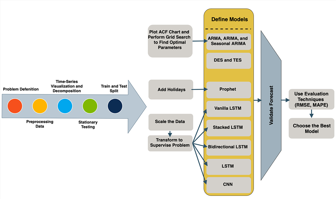
In recent years, there has been growing interest in the field of Neural Networks. However, research into seasonal time-series forecasting, which has many real-world applications, has produced varied results. In this repository, the performance of Neural Network methods in seasonal time-series forecasting has been compared with other methods. I began with some classical time-series forecasting methods like Seasonal ARIMA and Triple Exponential Smoothing. Then I tested more current methods like Prophet, Long Short-Term Memory (LSTM), and Convolutional Neural Network (CNN). The process is illustrated below.
The dataset used for this project describes Superstore Sales from 2014 to the end of 2017 and it contains nearly 10,000 observations and 21 features. This dataset consists of sales information of three different categories, furniture, technology, and office supplies. In this project, the sales of furniture is the variable of interest because it contains seasonal patterns. This dataset is publicly available and the most important features for performing univariate forecasting are sales and order date of each data point. Some of the other features are: Order ID, Order Date, Ship Date, Ship Mode, Customer ID, Customer Name, Segment, Country, City, State, Postal Code, Region, Category, Sub-Category, Product Name, Sales, Quantity, Discount, Profit.
There are many methods for evaluating a model, but in this research, the model performance is judged by the most commonly used measures. MSE, RMSE, and MAPE have been used to evaluate each method and select the best one among them. Mean Squared Error (MSE) measures the average of the squared predicted error values and Root Mean Squared Error (RMSE) is the standard deviation of the prediction errors and it is scale-dependent. Therefore, it cannot be used to compare time- series with different units. Mean Absolute Percentage Error (MAPE) calculates the mean absolute percentage error function for the forecast and the eventual outcomes.
For the task of time-series forecasting we cannot divide the dataset to train set and test set randomly. In fact, observations in time-series are dependent on each other and data should be split in time. Therefore, common techniques such as K-fold cross validation don’t work for time-series data. For the purposes of this project, I opted to use the first three years of sales data as the training set, and the remainder as the test set. This breaks down as 75% and 25%, respectively.
In order to gain a better insight of the dataset and to be able to predict future sales more accurate, it has been divided to three parts based on product categories, which are furniture, technology products, and office supplies. Then, the sales data has been aggregated by order date. In the next step, the data has been resampled on monthly frequency and averages daily sales value has been used. In addition, the start of the month has been set as the index.
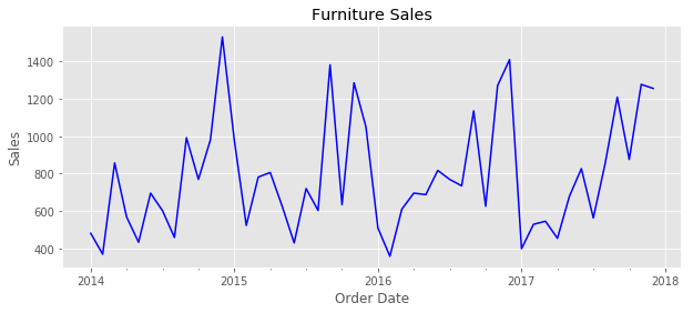
As it can be seen from the above figure, the furniture sales graph shows seasonality in its pattern. Sales volume is low at the start of each year and it increases at the end of the year. One of the main goals of this project is to investigate the performance of different forecasting methods on seasonal items and for this reason, the furniture products are going to be the chosen category for the task of prediction.
In this notebook, ARMA, ARIMA, and SARIMA methods are implemented using statsmodels library.
Auto Regressive Moving Average (ARMA) has been produced by combining the Autoregressive model and Moving Average model. This method can be applied on univariate time- series with no trend and seasonal components in their pattern and can be shown as ARMA (p, q) where p represents the order of the AR part and q is the order of the MA part.
Autoregressive Integrated Moving Average (ARIMA) is one of the most commonly used methods for time-series forecasting which consists of the combination of autoregressive models and moving average models and is usually applied on non-stationary time-series because of its ability to make the sequence stationary.
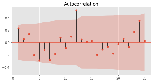
For predicting a seasonal time-series, Seasonal ARIMA or SARIMA model is used and it is denoted by SARIMA(p, d, q)(P,D,Q)m, where p, d, and q are non-seasonal and P, D, and Q are seasonal parameters and receptively they present order of the autoregressive part, degree of the first differencing, and order of the moving average part. In addition, the seasonal parameter m can be defined as the length of the cycle or in other words, the number of periods per season. This number can be found from the peaks of the ACF plots. As it has been shown in the following figure.
The method for identifying the optimal parameters is called the Grid Search method. Grid search will find the best hyper-parameters of the model by searching over the set of possible parameters and comparing the Akaike information criterion (AIC) and Bayesian information criterion (BIC) which are the estimators that can indicate the quality of the model. After finding all the parameters, the model can be created and fit on the training data and then can be used to make a prediction. After applying Grid search method, the best hyper-parameters for ARIMA and Seasonal ARIMA have been indicated as (6,0,0) and (0, 0, 0) x (1, 1, 0, 12) respectively.
Another popular time-series forecasting method is Exponential smoothing. This model can detect trends and seasonality and it is similar to the ARIMA method. However, instead of using the weighted linear sum of past data points, it assigns an exponentially decreasing weight to each observation. Exponential Smoothing can be divided into three main categories. Single Exponential Smoothing (SES) for forecasting univariate data without a trend or seasonality. Double Exponential Smoothing (DES) which supports trends in the time-series and Triple Exponential Smoothing (TES) which can handle seasonality as well. In this project the last two methods, DES and TES have been used to predict the furniture sales of a retail store.
Prophet is an open-sourced time-series forecasting model which has been introduced by Facebook recently. This model is based on an additive model which is capable of making high-quality forecasts from hourly, daily or weekly time-series that have at least a few months’ history. It can also predict the future pattern of time-series which contains historical trend fluctuations, and a large number of outliers or missing values. The first step in this approach is modelling the time-series with specified parameters. Then start the forecasting and then the performance will be evaluated. In the next step, if the results show poor performance, the problems will be informed to human analyst so they can adjust the model.
The last step before starting to fit the model is to change the name of the dataset’s columns. In order to work with Prophet, the date column should be changed to “ds” and the variable of interest should be changed to y. After that, the model can be generated and fit on the training data. After fitting the model and making the forecast, the result of forecast appears as a data-frame which includes lots of columns like yhat, which is the actual predicted value, yhat_lower and yhat_upper which indicate the uncertainty level.
One of the most popular proposed methods for time-series forecasting is the Recurrent Neural Networks (RNN) approach. RNN's ability to keep events from the past in its memory can be very useful in time-series forecasting. The issue with RNN is that after passing many hidden layers due to the multiplication the result is going to vanish or in other words, vanishing gradient or exploding gradient will happen. Long Short-Term Memory networks (LSTM) is a solution for short term memory of RNN and is trained to use back-propagation overtime to overcome the vanishing gradient problem.
In this project, four different LSTM models for time-series forecasting have been used. The first one is Vanilla LSTM which consists of a single hidden layer of LSTM and one layer of output. The second LSTM model is called Stacked LSTM and consists of multiple LSTM on top of each other. The third LSTM model is called bidirectional LSTM and learns the input sequence forward and backward by wrapping the first hidden layer in a layer called Bidirectional. The goal of using the fourth LSTM model in this project was to explore the effectiveness of a few changes in this method which is similar to the Vanilla LSTM model.
Finally, a Convolutional Neural Network (CNN) has been used. CNN is a class of deep neural networks which consists of one or more convolutional layers and it mainly used for image processing. However, because of its ability to identify patterns, it can be utilized in time-series forecasting as well. In this notebook a 1D CNN model has been proposed which consists of 3 one-dimensional convolution with 128 filters which describes the number of sliding windows that convolve across the data. The result from previous CNN will be fed into the next CNN layer. Followed by that there is the max-pooling layer that takes the maximum number in the sliding window and will prevent the model from overfitting. Also, between this layer and dense layer, a flatten layer has been used to reduce feature maps.
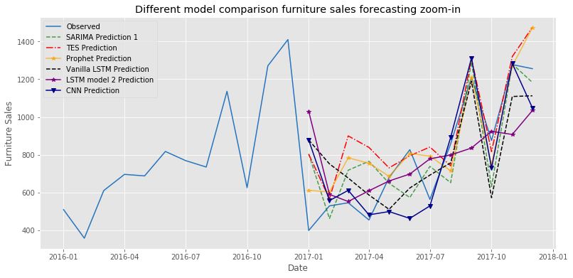
In this notebook, by implementing all of the previous models, the effectiveness of Neural Network methods on forecasting seasonal items has been explored and the results have been compared to each other. The following figure illustrates the predicted results of the best models from each forecasting technique. They have produced mixed results in the sales prediction for the beginning of the year but all of them could capture the growth in the sales at the end of the year 2017.
The following table shows the MSE, RMSE, and MAPE values for all of the models. As can be seen, the first SARIMA model outperformed other classical methods in terms of forecasting accuracy in different performance measurements. Furthermore, the holiday factor has improved the forecasting accuracy of the second Prophet model compared with the first model and also it has been performed better than the SARIMA model. Among the Neural networks models, the results show the good performance of Stacked LSTM, Vanilla LSTM, and CNN models compared with other methods. The results also indicate the superiority of Stacked LSTM over other methods with the MAPE value of 17.34 and the RMSE value of 128.51.
| Model | MSE | RMSE | MAPE |
|---|---|---|---|
| ARMA | 87,237.01 | 295.36 | 33.88 |
| ARIMA | 79,804.31 | 282.5 | 35.07 |
| SARIMA 1 | 42,305.37 | 205.68 | 28.89 |
| SARIMA 2 | 55,497.86 | 235.58 | 33.5 |
| DES | 40,4596.36 | 636.08 | 98.79 |
| TES | 49,846.48 | 223.26 | 30.81 |
| Prophet1 | 37,992.52 | 194.92 | 26.67 |
| Prophet2 | 27,986.56 | 167.29 | 22.62 |
| Vanilla LSTM | 18,829.66 | 137.22 | 18.39 |
| Stacked LSTM | 16,515.49 | 128.51 | 17.34 |
| Bidirectional LSTM | 53,981.32 | 232.34 | 31.4 |
| LSTM 1 | 68,671.5 | 262.05 | 29.4 |
| CNN | 39,938.47 | 199.85 | 22.26 |
