Coder Social home page Coder Social logo

spsanderson / healthyr.ts Goto Github PK

View Code? Open in Web Editor NEW
17.0 6.0 3.0 315.1 MB

A time-series companion package to healthyR

Home Page: https://www.spsanderson.com/healthyR.ts/

License: Other

R 99.73% Rez 0.27%
time-series modeling forecasting r r-package rstats ggplot2 machine-learning arima-forecasting arima-model

healthyr.ts's Introduction

healthyR.ts

CRAN_Status_Badge Lifecycle: experimental PRs Welcome

The goal of healthyR.ts is to provide a consistent verb framework for performing time series analysis and forecasting on both administrative and clinical hospital data.

Installation

You can install the released version of healthyR.ts from CRAN with:

install.packages("healthyR.ts")

And the development version from GitHub with:

# install.packages("devtools")
devtools::install_github("spsanderson/healthyR.ts")

Example

This is a basic example which shows you how to generate random walk data.

library(healthyR.ts)
library(ggplot2)

df <- ts_random_walk()

head(df)
#> # A tibble: 6 × 4
#>     run     x        y cum_y
#>   <dbl> <dbl>    <dbl> <dbl>
#> 1     1     1  0.0541  1054.
#> 2     1     2 -0.143    904.
#> 3     1     3 -0.0285   878.
#> 4     1     4  0.245   1093.
#> 5     1     5  0.0658  1165.
#> 6     1     6  0.00266 1168.

Now that the data has been generated, lets take a look at it.

df %>%
   ggplot(
       mapping = aes(
           x = x
           , y = cum_y
           , color = factor(run)
           , group = factor(run)
        )
    ) +
    geom_line(alpha = 0.8) +
    ts_random_walk_ggplot_layers(df)

That is still pretty noisy, so lets see this in a different way. Lets clear this up a bit to make it easier to see the full range of the possible volatility of the random walks.

library(dplyr)
library(ggplot2)

df %>%
    group_by(x) %>%
    summarise(
        min_y = min(cum_y),
        max_y = max(cum_y)
    ) %>%
    ggplot(
        aes(x = x)
    ) +
    geom_line(aes(y = max_y), color = "steelblue") +
    geom_line(aes(y = min_y), color = "firebrick") +
    geom_ribbon(aes(ymin = min_y, ymax = max_y), alpha = 0.2) +
    ts_random_walk_ggplot_layers(df)

This package comes with a wide variety of functions from Data Generators to Statistics functions. The function ts_random_walk() in the above example is a Data Generator.

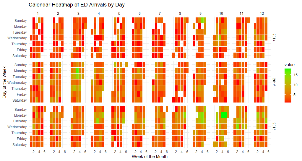
Let’s take a look at a plotting function.

data_tbl <- data.frame(
  date_col = seq.Date(
    from = as.Date("2020-01-01"),
    to   = as.Date("2022-06-01"),
    length.out = 365*2 + 180
    ),
  value = rnorm(365*2+180, mean = 100)
)

ts_calendar_heatmap_plot(
  .data          = data_tbl
  , .date_col    = date_col
  , .value_col   = value
  , .interactive = FALSE
)

Time Series Clustering via Features:

data_tbl <- ts_to_tbl(AirPassengers) %>%
  mutate(group_id = rep(1:12, 12))

output <- ts_feature_cluster(
  .data = data_tbl,
  .date_col = date_col,
  .value_col = value,
  group_id,
  .features = c("acf_features","entropy"),
  .scale = TRUE,
  .prefix = "ts_",
  .centers = 3
)

ts_feature_cluster_plot(
  .data = output,
  .date_col = date_col,
  .value_col = value,
  .center = 2,
  group_id
)

Time to/from Event Analysis

library(dplyr)
df <- ts_to_tbl(AirPassengers) %>% select(-index)

ts_time_event_analysis_tbl(
  .data = df,
  .horizon = 6,
  .date_col = date_col,
  .value_col = value,
  .direction = "both"
) %>%
  ts_event_analysis_plot()

ts_time_event_analysis_tbl(
  .data = df,
  .horizon = 6,
  .date_col = date_col,
  .value_col = value,
  .direction = "both"
) %>%
  ts_event_analysis_plot(.plot_type = "individual")

ARIMA Simulators

output <- ts_arima_simulator()
output$plots$static_plot

Automatic Workflows which can be thought of as Boiler Plate Time Series modeling. This is in it’s infancy in this package.

Auto Workflows Boilerplate Workflow
ts_auto_arima() Boilerplate Workflow
ts_auto_arima_xgboost() Boilerplate Workflow
ts_auto_croston() Boilerplate Workflow
ts_auto_exp_smoothing() Boilerplate Workflow
ts_auto_glmnet() Boilerplate Workflow
ts_auto_lm() Boilerplate Workflow
ts_auto_mars() Boilerplate Workflow
ts_auto_nnetar() Boilerplate Workflow
ts_auto_prophet_boost() Boilerplate Workflow
ts_auto_prophet_reg() Boilerplate Workflow
ts_auto_smooth_es() Boilerplate Workflow
ts_auto_svm_poly() Boilerplate Workflow
ts_auto_svm_rbf() Boilerplate Workflow
ts_auto_theta() Boilerplate Workflow
ts_auto_xgboost() Boilerplate Workflow

This is just a start of what is in this package!

healthyr.ts's People

Contributors

emilhvitfeldt avatar hfrick avatar olivroy avatar spsanderson avatar

Stargazers

 avatar  avatar  avatar  avatar  avatar  avatar  avatar  avatar  avatar  avatar  avatar  avatar  avatar  avatar  avatar  avatar

Watchers

 avatar  avatar  avatar  avatar  avatar  avatar

healthyr.ts's Issues

New function `ts_splits_plot`

Takes in a splits object and plots out the cv using the timetk functions. This is a simple wrapper to obtain the plot.

splits <- time_series_split(data_prepared_tbl, assess = "8 weeks", cumulative = TRUE)

splits %>%
    tk_time_series_cv_plan() %>%
    plot_time_series_cv_plan(optin_time, optins_trans)

Should turning into something like:

splits <- time_series_split(data_tbl, assess = "8 weeks", cumulative = TRUE)

ts_splits_plot(.splits_obj = splits, .date_col = date_col, .value_col = value)

Two Sided Moving Average Plot `ts_two_sided_ma_plot`

This function should return a two-sided moving average plot.

library(healthyR.data)
library(dplyr)
library(timetk)


data_tbl <- healthyR_data%>%
    filter(ip_op_flag == 'I') %>%
    summarise_by_time(
        .date_var = visit_end_date_time,
        .by = "month",
        value = n()
    ) %>%
    filter_by_time(
        .date_var = visit_end_date_time,
        .start_date = "2015",
        .end_date = "2019"
    ) %>%
    rename(date_col = visit_end_date_time)

ts_two_sided_ma_plot(.data, .date_col, .value_col, .interactive)

Release healthyR.ts 0.1.3

Prepare for release:

Submit to CRAN:

  • usethis::use_version('patch')
  • devtools::submit_cran()
  • Approve email

Wait for CRAN...

  • Accepted 🎉
  • usethis::use_github_release()
  • usethis::use_dev_version()

Add functions for workflow set type integration

Make a function that will take in a list of preprocessors and the data argument that will then produce an algorithm-specific workflow_sets object that gets passed to modeltime calibrate for sets and returns a list object

Add the following Algorithms from modeltime:

  • linear_reg()
  • mars
  • svm_poly
  • svm_rbf

`tidy` style function for Fourier Analysis

Tidy the below:

Add a column of harmonic number

Make the output a list object

See SO https://stackoverflow.com/questions/41435777/perform-fourier-analysis-to-a-time-series-in-r#41465250

Code:

library(healthyR.data)
library(tidyverse)
library(timetk)

dat   <- healthyR_data%>%
  filter(ip_op_flag == 'I') %>%
  summarise_by_time(
    .date_var = visit_end_date_time,
    .by = "month",
    V1 = n()
  ) %>%
  filter_by_time(
    .date_var = visit_end_date_time,
    .start_date = "2015",
    .end_date = "2019"
  )
y     <- dat$V1
data_len <- nrow(dat)
t     <- 1:data_len
rg    <- diff(range(y))

nff = function(x = NULL, n = NULL, up = 10L, plot = TRUE, add = FALSE, main = NULL, ...){
  #The direct transformation
  #The first frequency is DC, the rest are duplicated
  dff = fft(x)
  #The time
  t = seq(from = 1, to = length(x))
  #Upsampled time
  nt = seq(from = 1, to = length(x)+1-1/up, by = 1/up)
  #New spectrum
  ndff = array(data = 0, dim = c(length(nt), 1L))
  ndff[1] = dff[1] #Always, it's the DC component
  if(n != 0){
    ndff[2:(n+1)] = dff[2:(n+1)] #The positive frequencies always come first
    #The negative ones are trickier
    ndff[length(ndff):(length(ndff) - n + 1)] = dff[length(x):(length(x) - n + 1)]
  }
  #The inverses
  indff = fft(ndff/data_len, inverse = TRUE)
  idff = fft(dff/data_len, inverse = TRUE)
  if(plot){
    if(!add){
      plot(x = t, y = x, pch = 16L, xlab = "Time", ylab = "Measurement",
           main = ifelse(is.null(main), paste(n, "harmonics"), main))
      lines(y = Mod(idff), x = t, col = adjustcolor(1L, alpha = 0.5))
    }
    lines(y = Mod(indff), x = nt, ...)
  }
  ret = data.frame(time = nt, y = Mod(indff))
  return(ret)
}

colors = rainbow(36L, alpha = 0.3)
nff(x = y, n = 36L, up = 100L, col = colors[1])
png("all_waves.png")
for(i in 1:36){
  ad = ifelse(i == 1, FALSE, TRUE)
  nff(x = y, n = i, up = 60L, col = colors[i], add = ad, main = "All waves up to 36th harmonic")
}
dev.off()

all_waves

Make function `ts_model_spec_tuner`

ts_model_spec_tuner <- function(.parsnip_engine = NULL){
  
  # * Tidyeval ----
  pe <- base::as.character(.parsnip_engine)
  
  # * Checks ----
  if(!pe %in% c("auto_arima","auto_arima_xgboost",
    "ets","croston","theta",
    "stlm_ets","tbats","stlm_arima",
    "nnetar",
    "prophet","prophet_xgboost",
    "lm","glmnet","stan","spark","keras",
    "earth","xgboost")){
    stop(call. = FALSE, base::paste0("The parameter (.parsnip_engine) value of: ", pe, ", is not supported."))
  }
  
  if(pe %in% c("auto_arima","stlm_ets","tbats","stlm_arima")){
    stop(call. = FALSE, base::paste0("The parameter (.parsnip_engine) value of: ", pe, ", is an auto tuned model spec already."))
  }
  
  if(pe %in% c("lm")){
    stop(call. = FALSE, base::paste0("The parameter (.parsnip_engine) value of: ", pe, ", has no tuning parameters."))
  }
  
  # * Model Spec Tuner ----
  if (pe == "auto_arima_xgboost"){
    mst <- modeltime::arima_boost(
      trees            = tune::tune()
      , min_n          = tune::tune()
      , tree_depth     = tune::tune()
      , learn_rate     = tune::tune()
      , loss_reduction = tune::tune()
      , sample_size    = tune::tune()
      , stop_iter      = tune::tune()
    ) %>%
      parsnip::set_engine(pe)
  } else if (pe == "ets"){
    mst <- modeltime::exp_smoothing(
      seasonal_period = "auto"
      , error         = "auto"
      , trend         = "auto"
      , season        = "auto"
      , damping       = "auto"
      , smooth_level    = tune::tune()
      , smooth_trend    = tune::tune()
      , smooth_seasonal = tune::tune()
    ) %>%
      parsnip::set_engine(pe)
  } else if (pe == "croston"){
    mst <- modeltime::exp_smoothing(
      seasonal_period = "auto"
      , error         = "auto"
      , trend         = "auto"
      , season        = "auto"
      , damping       = "auto"
      , smooth_level    = tune::tune()
      , smooth_trend    = tune::tune()
      , smooth_seasonal = tune::tune()
    ) %>%
      parsnip::set_engine(pe)
  } else if (pe == "theta"){
    mst <- modeltime::exp_smoothing(
      seasonal_period = "auto"
      , error         = "auto"
      , trend         = "auto"
      , season        = "auto"
      , damping       = "auto"
      , smooth_level    = tune::tune()
      , smooth_trend    = tune::tune()
      , smooth_seasonal = tune::tune()
    ) %>%
      parsnip::set_engine(pe)
  } else if (pe == "nnetar"){
    mst <- modeltime::nnetar_reg(
      seasonal_period   = "auto"
      , non_seasonal_ar = tune::tune()
      , seasonal_ar     = tune::tune()
      , hidden_units    = tune::tune()
      , num_networks    = tune::tune()
      , penalty         = tune::tune()
      , epochs          = tune::tune()
    ) %>%
      parsnip::set_engine(pe)
  } else if (pe == "prophet"){
    mst <- modeltime::prophet_reg(
      changepoint_num      = tune::tune()
      , changepoint_range  = tune::tune()
      , seasonality_yearly = "auto"
      , seasonality_weekly = "auto"
      , seasonality_daily  = "auto"
      , prior_scale_changepoints = tune::tune()
      , prior_scale_seasonality  = tune::tune()
      , prior_scale_holidays     = tune::tune()
    ) %>%
      parsnip::set_engine(pe)
  } else if (pe == "prophet_xgboost"){
    mst <- modeltime::prophet_boost(
      changepoint_num      = tune::tune()
      , changepoint_range  = tune::tune()
      , seasonality_yearly = FALSE
      , seasonality_weekly = FALSE
      , seasonality_daily  = FALSE
      , prior_scale_changepoints = tune::tune()
      , prior_scale_seasonality  = tune::tune()
      , prior_scale_holidays     = tune::tune()
      , trees                    = tune::tune()
      , min_n                    = tune::tune()
      , tree_depth               = tune::tune()
      , learn_rate               = tune::tune()
      , loss_reduction           = tune::tune()
      , sample_size              = tune::tune()
      , stop_iter                = tune::tune()
    ) %>%
      parsnip::set_engine(pe)
  } else if (pe == "glmnet") {
    mst <- parsnip::linear_reg(
      penalty   = tune::tune()
      , mixture = tune::tune()
    ) %>%
      parsnip::set_engine(pe)
  } else if (pe == "stan"){
    mst <- parsnip::linear_reg() %>%
      parsnip::set_engine(
        engine   = pe
        , chains = tune::tune()
        , iter   = tune::tune()
        , seed   = 123
      )
  } else if (pe == "spark"){
    mst <- parsnip::linear_reg(
      penalty   = tune::tune()
      , mixture = tune::tune()
    ) %>%
      parsnip::set_engine(pe)
  } else if (pe == "keras"){
    mst <- parsnip::linear_reg(
      penalty   = tune::tune()
      , mixture = tune::tune()
    ) %>%
      parsnip::set_engine(pe)
  } else if (pe == "earth"){
    mst <- parsnip::mars(
      num_terms = tune::tune()
      , prod_degree = tune::tune()
    ) %>%
      parsnip::set_engine(pe)
  } else if (pe == "xgboost"){
    mst <- parsnip::boost_tree(
      mtry             = tune::tune()
      , trees          = tune::tune()
      , min_n          = tune::tune()
      , tree_depth     = tune::tune()
      , learn_rate     = tune::tune()
      , loss_reduction = tune::tune()
      , sample_size    = tune::tune()
    ) %>%
      parsnip::set_engine(pe)
  }
  
  # * Return ----
  return(mst)
  
}

Release healthyR.ts 0.1.2

Prepare for release:

Submit to CRAN:

  • usethis::use_version('patch')
  • devtools::submit_cran()
  • Approve email

Wait for CRAN...

  • Accepted 🎉
  • usethis::use_github_release()
  • usethis::use_dev_version()

Function to grab comparison data

Given a day set grab data from same time period of n periods before

Example:
compare_time(start = 2020-01-01,
end = 2020-01-31, periods_back = 2)

This would give data from 2020-01-31 to 2020-01-31 and from 2018-01-01 to 2018-01-31 to make a comparison between the two periods

Release healthyR.ts 0.1.0.9001

Prepare for release:

  • devtools::build_readme()
  • Check current CRAN check results
  • devtools::check(remote = TRUE, manual = TRUE)
  • devtools::check_win_devel()
  • rhub::check_for_cran()
  • revdepcheck::revdep_check(num_workers = 4)
  • urlchecker::url_check()
  • Update cran-comments.md
  • Polish NEWS
  • Review pkgdown reference index for, e.g., missing topics
  • Draft blog post

Submit to CRAN:

  • usethis::use_version('minor')
  • devtools::submit_cran()
  • Approve email

Wait for CRAN...

  • Accepted 🎉
  • usethis::use_github_release()
  • usethis::use_dev_version()
  • Finish blog post
  • Tweet
  • Add link to blog post in pkgdown news menu

Make `ts_info_tbl` function

The function should return some basic information in tibble format about a given time series object. It should work as follows:

library(TSstudio)

ts_info_tbl(USgas)
# A tibble: 1 x 7
  name  class frequency start  end     var        length
  <chr> <chr>     <dbl> <chr>  <chr>   <chr>       <int>
1 USgas ts           12 2000 1 2019 10 univariate    238

ts_info_tbl(Coffee_Prices)
# A tibble: 1 x 7
  name          class frequency start  end    var         length
  <chr>         <chr>     <dbl> <chr>  <chr>  <chr>        <int>
1 Coffee_Prices mts          12 1960 1 2018 5 2 variables    701

ts_info_tbl(Michigan_CS)
# A tibble: 1 x 7
  name        class frequency start    end      var        length
  <chr>       <chr> <chr>     <chr>    <chr>    <chr>       <int>
1 Michigan_CS xts   monthly   Jan 1980 Dec 2019 1 variable    480

If the data is in a tibble format then the timetk::tk_summary_diganostics function should be used to return the same tibble of information if possible.

Function so far:

ts_info_tbl <- function(.data){
  
  # Internal Data Var ----
  ts_obj <- .data
  
  # * Checks ----
  if(!stats::is.ts(ts_obj) & !xts::is.xts(ts_obj) & !zoo::is.zoo(ts_obj)){
    stop(call. = FALSE, "(.data) must be a valid time series object, ts, xts, mts, or zoo.")
  }
  
  ts_name <- NULL
  ts_info <- NULL
  
  # Get Name
  ts_name <- base::deparse(base::substitute(.data))
  
  # * TS Object Tyep ----
  # ** Stats TS Object ----
  if(stats::is.ts(ts_obj) & !is.mts(ts_obj)){
    ts_info  <- tibble::tibble(
      name = ts_name,
      class = "ts",
      frequency = stats::frequency(ts_obj),
      start = base::paste(stats::start(ts_obj), collapse = " "),
      end = base::paste(stats::end(ts_obj), collapse = " "),
      var = "univariate",
      length = base::length(ts_obj)
    )
  } else if(stats::is.ts(ts_obj) & stats::is.mts(ts_obj)){
    ts_info <- tibble::tibble(
      name = ts_name,
      class = "mts",
      frequency = stats::frequency(ts_obj),
      start = base::paste(stats::start(ts_obj), collapse = " "),
      end = base::paste(stats::end(ts_obj), collapse = " "),
      var = base::paste(dim(ts_obj)[2], "variables", sep = " "),
      length = base::dim(ts_obj)[1],
    )
  } else if(xts::is.xts(ts_obj)){
    ts_info <- tibble::tibble(
      name = ts_name,
      class = "xts",
      frequency = dplyr::case_when(
        xts::periodicity(ts_obj)$scale != "minute" ~ xts::periodicity(ts_obj)$scale
        , TRUE ~ base::paste(xts::periodicity(ts_obj)$frequency, xts::periodicity(ts_obj)$units, collapse = " ")
      ),
      start = base::paste(stats::start(ts_obj), collapse = " "),
      end = base::paste(stats::end(ts_obj), collapse = " "),
      var = if(base::is.null(base::dim(ts_obj)) & !base::is.null(base::length(ts_obj))){
        "univariate"
      } else if(dim(ts_obj)[2] == 1){
        base::paste(dim(ts_obj)[2], "variable", sep = " ")
      } else if (dim(ts_obj)[2] > 1){
        base::paste(dim(ts_obj)[2], "variables", sep = " ")
      },
      length = if(base::is.null(base::dim(ts_obj)) & !base::is.null(base::length(ts_obj))){
        base::length(ts_obj)
      } else {
        base::dim(ts_obj)[1]
      }
    )
  } else if(zoo::is.zoo(ts_obj)){
    ts_info <- tibble::tibble(
      name = ts_name,
      class = "zoo",
      frequency = xts::periodicity(ts_obj)$scale,
      start = base::paste(stats::start(ts_obj), collapse = " "),
      end = base::paste(stats::end(ts_obj), collapse = " "),
      var = if(base::is.null(base::dim(ts_obj)) & !base::is.null(base::length(ts_obj))){
        "univariate"
      } else if(dim(ts_obj)[2] == 1){
        base::paste(dim(ts_obj)[2], "variable", sep = " ")
      } else {
        base::paste(dim(ts_obj)[2], "variables", sep = " ")
      },
      length = if(base::is.null(base::dim(ts_obj)) & !base::is.null(base::length(ts_obj))){
        base::length(ts_obj)
      } else if(dim(ts_obj)[2] == 1){
        base::dim(ts_obj)[1]
      } else {
        base::length(ts_obj)
      }
    )
  }
  
  # * Return ----
  return(ts_info)
}

Add `ts_calendar_heatmap_plt()` functionality

Function should take in an aggregated data.frame / tibble and return either a plotly plot or a ggplot calendar heatmap.

Working example (maybe return invisible)

library(tidyverse)
library(timetk)
library(lubridate)
library(zoo)
library(healthyR.data)
library(stringi)
library(plotly)

data <- healthyR_data %>%
    filter(ip_op_flag == "O") %>%
    filter(substr(visit_id, 1, 1) == "8") %>%
    select(visit_start_date_time) %>%
    filter_by_time(
        .date_var     = visit_start_date_time
        , .start_date = "2014"
        , .end_date   = "2016"
    ) %>%
    summarise_by_time(
        .date_var = visit_start_date_time
        , value   = n()
    ) %>%
    set_names("date_col","value") %>%
    tk_augment_timeseries_signature(.date_var = date_col) %>%
    select(
        date_col
        , value
        , year
        , month
        , week
        , wday.lbl
    ) %>%
    mutate(yearmonth_fct = as.yearmon(date_col) %>% factor()) %>%
    mutate(wday.lbl = fct_rev(wday.lbl)) %>%
    select(date_col, year, yearmonth_fct, everything()) %>%
    arrange(date_col) %>%
    mutate(week_of_month = stri_datetime_fields(date_col)$WeekOfMonth) %>%
    rename("week_day" = "wday.lbl")

g <- ggplot(
        data = data
        , aes(
            x = week_of_month
            , y = week_day
            , fill = value
        )
    ) +
    geom_tile(color = "white") +
    facet_grid(year ~ month) +
    scale_fill_gradient(low = "red", high = "green") +
    labs(
        title = "Calendar Heatmap of ED Arrivals by Day"
        , x = "Week of the Month"
        , y = "Day of the Week"
    ) +
    theme_minimal()

print(g)
ggplotly(g)

Example plot:

Rplot

Sample Code:

#' Time Series Calendar Heatmap
#'
#' @author Steven P. Sanderson II, MPH
#'
#' @description
#' Takes in data that has been aggregated to the day level and makes a calendar
#' heatmap.
#'
#' @details
#' The data provided must have been aggregated to the day level, if not funky
#' output could result and it is possible nothing will be output but errors.
#' There must be a date column and a value column, those are the only items
#' required for this function to work.
#'
#' This function is intentionally inflexible, it complains more and does less in
#' order to force the user to supply a clean data-set.
#'
#' @param .data The time-series data with a date column and value column.
#' @param .date_col The column that has the datetime values
#' @param .value_col The column that has the values
#' @param .low The color for the low value, must be quoted like "red". The default is "red"
#' @param .high The color for the high value, must be quoted like "green". The default is "green"
#' @param .plt_title The title of the plot
#' @param .interactive Default is TRUE to get an interactive plot using [plotly::ggplotly()].
#' It can be set to FALSE to get a ggplot plot.
#'
#' @examples
#' library(LICHospitalR)
#' library(tidyverse)
#' library(timetk)
#' library(lubridate)
#' library(zoo)
#' library(scales)
#'
#' data_tbl <- ts_ed_arrivals_query() %>%
#'   ts_ed_arrivals_tbl(.date_col = date_col, .by_time = "day") %>%
#'   filter_by_time(.date_var = date_col, .start_date = "2021") %>%
#'   set_names("date_col","value")
#'
#' ts_calendar_heatmap_plt(
#'   .data        = data_tbl
#'   , .date_col  = date_col
#'   , .value_col = value
#' )
#'
#' ts_calendar_heatmap_plt(
#'   .data          = data_tbl
#'   , .date_col    = date_col
#'   , .value_col   = value
#'   , .interactive = FALSE
#' )
#'
#' @return
#' A ggplot2 plot or if interactive a plotly plot
#'
#' @export
#'

ts_calendar_heatmap_plt <- function(.data, .date_col, .value_col,
                                    .low = "red", .high = "green",
                                    .plt_title = "",
                                    .interactive = TRUE){

  # * Tidyeval ----
  date_col_var_expr  <- rlang::enquo(.date_col)
  value_col_var_expr <- rlang::enquo(.value_col)
  plotly_plt         <- .interactive
  low                <- .low
  high               <- .high

  # * Checks ----
  if (rlang::quo_is_missing(date_col_var_expr)) {
    stop(call. = FALSE, "(.date_col) is missing, please supply.")
  }

  if (rlang::quo_is_missing(value_col_var_expr)){
    stop(call. = FALSE, "(.value_col) is missing, please supply.")
  }

  if(!is.logical(plotly_plt)){
    stop(call. = FALSE, "You must supply either TRUE or FALSE for .interactive")
  }

  # * Data and Manipulation ----
  data <- tibble::as_tibble(.data) %>%
    dplyr::select( {{date_col_var_expr }}, {{ value_col_var_expr }} ) %>%
    purrr::set_names("date_col", "value")

  data_tbl <- data %>%
    LICHospitalR::ts_ymwdh_tbl(date_col) %>%
    #dplyr::mutate(yearmonth_fct <- zoo::as.yearmon(date_col) %>% base::factor()) %>%
    dplyr::mutate(week_day = forcats::fct_rev(wd)) %>%
    dplyr::select(date_col, yr, dplyr::everything()) %>%
    dplyr::arrange(date_col) %>%
    dplyr::mutate(week_of_month = stringi::stri_datetime_fields(date_col)$WeekOfMonth)

  # * Plot ----
  g <- ggplot2::ggplot(
    data = data_tbl
    , ggplot2::aes(
      x      = week_of_month
      , y    = week_day
      , fill = value
    )
  ) +
    ggplot2::geom_tile(color = "white") +
    ggplot2::facet_grid(yr ~ mn) +
    ggplot2::scale_fill_gradient(low = low, high = high) +
    ggplot2::labs(
      title = .plt_title
    )
    ggplot2::theme_minimal()

  # Which plot to return
  if(plotly_plt){
    plt <- plotly::ggplotly(g)
  } else {
    plt <- g
  }

  # * Return ----
  print(plt)

}

Compare Time function

Given a data set grab data from the same time period of n periods before

Example:
compare_time(start = 2020-01-01,
end = 2020-01-31, periods_back = "2 years")

This would give data from 2020-01-31 to 2020-01-31 and from 2018-01-01 to 2018-01-31 to make a comparison between the two periods

onAttach message

make a message for library() .onAttach()

Similar to bayesmodels

.onAttach <- function(libname, pkgname) {

bsu_rule_color <- "#2c3e50"
bsu_main_color <- "#1f78b4"

# Check Theme: If Dark, Update Colors
tryCatch({
    if (rstudioapi::isAvailable()) {
        theme <- rstudioapi::getThemeInfo()
        if (is.null(theme)) {
            bsu_rule_color <- "#2c3e50"
            bsu_main_color <- "#1f78b4"
        }
        if (theme$dark) {
            bsu_rule_color <- "#7FD2FF"
            bsu_main_color <- "#18bc9c"
        }
    }
}, error = function(e) {
    bsu_rule_color <- "#2c3e50"
    bsu_main_color <- "#1f78b4"
}, finally = {
    bsu_main <- crayon::make_style(bsu_main_color)
    
    msg <- paste0(
        cli::rule(left = "Welcome to bayesmodels", col = bsu_rule_color, line = 2),
        bsu_main('\nIf you are interested in time series, maybe you would like to check my other packages: garchmodels and boostime\n'),
        bsu_main('</> If you find this package useful, please leave a star: https://github.com/AlbertoAlmuinha/bayesmodels </>')
    )
    
    packageStartupMessage(msg)
})

}

Make a model tuner function `ts_model_tune()`

ts_model_tune <- function(.modeltime_model_id, .calibration_tbl,
                          .splits_obj, .drop_training_na = TRUE, .date_col,
                          .value_col, .tscv_assess = "12 months", 
                          .tscv_skip = "6 months", .slice_limit = 6,
                          .facet_ncol = 2, .grid_size = 30, .num_cores = 1,
                          .best_metric = "rmse") {
  
  # * Tidyeval ----
  model_number    <- base::as.integer(.modeltime_model_id)
  calibration_tbl <- .calibration_tbl
  splits_obj      <- .splits_obj
  drop_na         <- base::as.logical(.drop_training_na)
  date_col        <- rlang::enquo(.date_col)
  value_col       <- rlang::enquo(.value_col)
  assess          <- .tscv_assess
  skip            <- .tscv_skip
  slice_limit     <- .slice_limit
  facet_ncol      <- base::as.integer(.facet_ncol)
  grid_size       <- base::as.integer(.grid_size)
  num_cores       <- base::as.integer(.num_cores)
  best_metric     <- base::as.character(.best_metric)
  
  
  # * Checks ----
  if(!modeltime::is_calibrated(calibration_tbl)){
    stop(call. = FALSE, "(.calibration_tbl) must be a calibrated modeltime_table.")
  }
  
  if(!is.integer(model_number)){
    stop(call. = FALSE, "(.modeltime_model_id) must be an integer.")
  }
  
  # * Manipulations ----
  # Get Model
  plucked_model <- calibration_tbl %>%
    modeltime::pluck_modeltime_model(model_number)
  
  # Get Training Data
  if(!drop_na){
    training_data <- rsample::training(splits_obj)
  } else {
    training_data <- rsample::training(splits_obj) %>%
      tidyr::drop_na()
  }
  
  # Make TSCV
  tscv <- timetk::time_series_cv(
    data        = training_data,
    date_var    = {{ date_col }},
    cumulative  = TRUE,
    assess      = assess,
    skip        = skip,
    slice_limit = slice_limit
  )
  
  # TSCV Data Plan Tibble
  tscv_data_tbl <- tscv %>%
    timetk::tk_time_series_cv_plan()
  
  # TSCV Plot
  tscv_plt <- tscv_data_tbl %>%
    timetk::plot_time_series_cv_plan(
      {{ date_col }}, {{ value_col }}, .facet_ncol = {{ facet_ncol }}
    )
  
  # * Tune Spec ----
  # Model Spec
  model_spec        <- plucked_model %>% parsnip::extract_spec_parsnip()
  model_spec_engine <- model_spec[["engine"]]
  model_spec_tuner  <- ts_model_spec_tuner(model_spec_engine)
  
  # * Grid Spec ----
  grid_spec <- dials::grid_latin_hypercube(
    tune::parameters(model_spec_tuner)
    , size = grid_size
  )
  
  # * Tune Model ----
  wflw_tune_spec <- plucked_model %>%
    workflows::update_model(model_spec_tuner)
  
  # * Run Tuning Grid ----
  modeltime::parallel_start(num_cores)
  
  tune_results <- wflw_tune_spec %>%
    tune::tune_grid(
      resamples = tscv
      , grid    = grid_spec
      , metrics = modeltime::default_forecast_accuracy_metric_set()
      , control = tune::control_grid(
        verbose     = TRUE
        , save_pred = TRUE
      )
    )
  
  modeltime::parallel_stop()
  
  # * Get best result
  best_result_set <- tune_results %>%
    tune::show_best(metric = best_metric, n = 1)
  
  # * Viz results ----
  tune_results_plt <- tune_results %>%
    tune::autoplot() +
    ggplot2::geom_smooth(se = FALSE)
  
  # * Retrain and Assess ----
  wflw_tune_spec_tscv <- wflw_tune_spec %>%
    workflows::update_model(model_spec_tuner) %>%
    tune::finalize_workflow(
      tune_results %>%
        tune::show_best(metric = best_metric, n = 1)
    ) %>%
    parsnip::fit(rsample::training(splits_obj))
  
  # * Calibration Tuned tibble ----
  calibration_tuned_tbl <- modeltime::modeltime_table(
    wflw_tune_spec_tscv
  ) %>%
    modeltime::modeltime_calibrate(rsample::testing(splits_obj))
  
  
  # * Return ----
  output <- list(
    data = list(
      calibration_tbl        = calibration_tbl,
      calibration_tuned_tbl  = calibration_tuned_tbl,
      tscv_data_tbl          = tscv_data_tbl,
      tuned_results          = tune_results,
      best_tuned_results_tbl = best_result_set,
      tscv_obj               = tscv
    ),
    model_info = list(
      model_spec          = model_spec,
      model_spec_engine   = model_spec_engine,
      model_spec_tuner    = model_spec_tuner,
      plucked_model       = plucked_model,
      wflw_tune_spec      = wflw_tune_spec,
      grid_spec           = grid_spec,
      wflw_tune_spec_tscv = wflw_tune_spec_tscv
    ),
    plots = list(
      tune_results_plt = tune_results_plt,
      tscv_plt         = tscv_plt
    )
  )

  return(output)
  
}

Release healthyR.ts 0.1.5

Prepare for release:

  • Check current CRAN check results
  • Polish NEWS
  • devtools::build_readme()
  • urlchecker::url_check()
  • devtools::check(remote = TRUE, manual = TRUE)
  • devtools::check_win_devel()
  • rhub::check_for_cran()
  • revdepcheck::revdep_check(num_workers = 4)
  • Update cran-comments.md

Submit to CRAN:

  • usethis::use_version('patch')
  • devtools::submit_cran()
  • Approve email

Wait for CRAN...

  • Accepted 🎉
  • usethis::use_github_release()
  • usethis::use_dev_version()

Add a function `ts_ma_plot`

Add a plot ts_ma_plot() that takes in the following arguments:

  • .data - is the data being supplied to the function
  • .date_col - is the column with the timestamp
  • .value_col - is the column with the value we want to plot and make transformations from
  • .ts_freqeuncy - is the frequency of the data that will get supplied internal to the function tk_ts() in character, default = "monthly" else "weekly" gets applied internally.
  • .plt_title - is the title of the main plot
  • .main_title - is the title of the top graph
  • .secondary_title - is the title of the second graph
  • .tertiary_title - is the title of the third graph

This should return a list object of the following items:

  1. data_trans_xts (an xts object with the original value and the monthly moving average)
  2. data_month_diff_xts (an xts object with the monthly difference in %)
  3. data_yoy_diff_xts (an xts object with the YoY growth %)
  4. data_summary_tbl (builds the ggplot2 version of the plot.xts object)
  5. pgrid (a cowplot object of the ggplot2 version of the plot.xts plot
  6. xts_plt (an xts plot object) generated from the internal function

A preview of the xts plot
Rplot

A preview of the ggplot2 plot
Rplot01

pseudo code to modify:

ts_ma_plot_test <- function(.data,
                            .date_col,
                            .value_col,
                            .ts_frequency = "monthly", 
                            .main_title = NULL,
                            .secondary_title = NULL,
                            .tertiary_title = NULL) {

  # * Tidyeval ----
  date_col_var_expr  <- rlang::enquo(.date_col)
  value_col_var_expr <- rlang::enquo(.value_col)
  ts_freq_var_expr   <- .ts_frequency
  ts_freq_for_calc   <- if(ts_freq_var_expr == "monthly"){
                          ts_freq_for_calc <- 12
                        } else {
                          ts_freq_for_calc <- round(365.25/7, 0)
                        }
  .main_title        <- .main_title
  .secondary_title   <- .secondary_title
  .tertiary_title    <- .tertiary_title

  # * Checks ----
  if (rlang::quo_is_missing(date_col_var_expr)) {
    stop(call. = FALSE, "(.date_col) is missing, please supply.")
  }

  if (rlang::quo_is_missing(value_col_var_expr)) {
    stop(call. = FALSE, "(.value_col) is mising, please supply.")
  }

  if (!is.data.frame(.data)) {
    stop(call. = FALSE, "(.data) is missing, please supply.")
  }

  if (is.null(ts_freq_var_expr)) {
    message(".ts_frequency was not supplied. One will try to be obtained.")
  }
  
  # * Data ----
  data_tbl <- tibble::as_tibble(.data) %>%
    dplyr::select({{ date_col_var_expr }}, {{ value_col_var_expr }}) %>%
    purrr::set_names("date_col", "value")

  # * Manipulate ----
  # Initial tables that get coerced to xts
  data_trans_tbl <- data_tbl %>%
    dplyr::mutate(
      ma12 = timetk::slidify_vec(
        .x = value,
        .period = ts_freq_for_calc,
        .f = mean,
        na.rm = TRUE
      )
    )

  data_diff_a <- data_trans_tbl %>%
    dplyr::mutate(diff_a = (value / dplyr::lag(value) - 1) * 100) %>%
    dplyr::select(date_col, diff_a)

  data_diff_b <- data_trans_tbl %>%
    dplyr::mutate(diff_b = (value / dplyr::lag(value, ts_freq_for_calc) - 1) * 100) %>%
    dplyr::select(date_col, diff_b)

  # Get start date for timetk::tk_ts() function
  start_date <- min(data_trans_tbl$date_col)
  start_yr <- lubridate::year(start_date)
  start_mn <- lubridate::month(start_date)

  # xts data
  data_trans_xts <- timetk::tk_ts(
    data_trans_tbl,
    frequency = ts_freq_for_calc,
    start = c(start_yr, start_mn)
  ) %>%
    timetk::tk_xts()

  data_diff_xts_a <- timetk::tk_ts(
    data_diff_a,
    frequency = ts_freq_for_calc,
    start = c(start_yr, start_mn)
  ) %>%
    xts::as.xts()

  data_diff_xts_b <- timetk::tk_ts(
    data_diff_b,
    frequency = ts_freq_for_calc,
    start = c(start_yr, start_mn)
  ) %>%
    xts::as.xts()

  # tibbles for ggplot/cowplot
  data_summary_tbl <- data_tbl %>%
    dplyr::mutate(date_col = as.Date(date_col)) %>%
    dplyr::mutate(
      ma12 = timetk::slidify_vec(
        .x = value,
        .period = ts_freq_for_calc,
        .f = mean,
        na.rm = TRUE
      )
    ) %>%
    dplyr::mutate(diff_a = (value / dplyr::lag(value) - 1) * 100) %>%
    dplyr::mutate(diff_b = (value / dplyr::lag(value, ts_freq_for_calc) - 1) * 100) %>%
    dplyr::mutate(
      diff_a = ifelse(is.na(diff_a), 0, diff_a),
      diff_b = ifelse(is.na(diff_b), 0, diff_b)
    )

  # * Visualize ----
  # ggplot only here, plot.xts in the list object
  p1 <- ggplot2::ggplot(
    data = data_summary_tbl,
    ggplot2::aes(
      x = date_col,
      y = value
    )
  ) +
    ggplot2::geom_line(size = 1) +
    ggplot2::geom_line(
      ggplot2::aes(
        x = date_col,
        y = ma12
      ),
      color = "blue",
      size = 1
    ) +
    ggplot2::scale_y_continuous(labels = scales::label_number_si()) +
    tidyquant::theme_tq() +
    ggplot2::labs(
      title = .main_title,
      x = "",
      y = ""
    ) +
    ggplot2::theme(
      axis.title.x = ggplot2::element_blank(),
      axis.text.x  = ggplot2::element_blank(),
      axis.ticks.x = ggplot2::element_blank()
    )

  p2 <- ggplot2::ggplot(
    data = data_summary_tbl,
    ggplot2::aes(
      x = date_col,
      y = diff_a,
      fill = ifelse(diff_a < 1, "red", "green")
    )
  ) +
    ggplot2::geom_col() +
    ggplot2::scale_y_continuous(
      labels = scales::label_percent(scale = 1, accuracy = 0.1)
    ) +
    tidyquant::theme_tq() +
    tidyquant::scale_fill_tq() +
    ggplot2::labs(
      title = .secondary_title,
      x = "",
      y = ""
    ) +
    ggplot2::theme(
      legend.position = "none",
      axis.title.x = ggplot2::element_blank(),
      axis.text.x = ggplot2::element_blank(),
      axis.ticks.x = ggplot2::element_blank()
    )

  p3 <- ggplot2::ggplot(
    data = data_summary_tbl,
    ggplot2::aes(
      x = date_col,
      y = diff_b,
      fill = ifelse(diff_b < 1, "red", "green")
    )
  ) +
    ggplot2::geom_col() +
    ggplot2::scale_y_continuous(
      labels = scales::label_percent(
        scale = 1,
        accuracy = 0.1
      )
    ) +
    ggplot2::scale_x_date(
      labels = scales::label_date("'%y"),
      breaks = scales::breaks_width("2 years")
    ) +
    tidyquant::theme_tq() +
    tidyquant::scale_fill_tq() +
    ggplot2::labs(
      title = .tertiary_title,
      x = "",
      y = ""
    ) +
    ggplot2::theme(
      legend.position = "none"
    )

  pgrid <- cowplot::plot_grid(
    # ggplots
    p1, p2, p3,
    ncol = 1,
    rel_heights = c(8, 5, 5)
  )

  # xts plot?
  ts_xts_plt_internal <- function(){
    plot.xts(
      data_trans_xts,
      main = .main_title,
      multi.panel = FALSE,
      col = c("black","blue")
    )
    lines(
      data_diff_xts_a,
      col = "red",
      type = "h",
      on = NA,
      main = .secondary_title
    )
    lines(
      data_diff_xts_b,
      col = "purple",
      type = "h",
      on = NA,
      main = .tertiary_title
    )
    addLegend(
      "bottomleft",
      on = 1,
      lty = c(1,1),
      lwd = c(2,1),
      col = c("black","blue")
    )
  }

  # * Return ----
  output <- list(
    data_trans_xts = data_trans_xts,
    data_diff_xts_a = data_diff_xts_a,
    data_diff_xts_b = data_diff_xts_b,
    data_summary_tbl = data_summary_tbl,
    pgrid = pgrid,
    xts_plt = ts_xts_plt_internal()
  )
  
  return(output)
  
}

Simple Moving Average plot `ts_sma_plot`

A plotting function ts_sma_plot gets a simple moving average of a provided order and plots it against the original data. This function should also allow for plotting multiple moving averages and should return a plotly::ggplotly if the parameter .interactive is set to TRUE

library(healthyR.data)
library(dplyr)
library(timetk)


data_tbl <- healthyR_data%>%
    filter(ip_op_flag == 'I') %>%
    summarise_by_time(
        .date_var = visit_end_date_time,
        .by = "month",
        value = n()
    ) %>%
    filter_by_time(
        .date_var = visit_end_date_time,
        .start_date = "2015",
        .end_date = "2019"
    ) %>%
    rename(date_col = visit_end_date_time)

ts_sma_plot(.date_var = date_col, .value_col = value, .sma_order = 4, .multiple_sma = FALSE, .interactve = FALSE)
ts_sma_plot(.date_var = date_col, .value_col = value, .sma_order = 4, .multiple_sma = TRUE, .interactive = TRUE)

Release healthyR.ts 0.1.1

Prepare for release:

  • Check that description is informative
  • Check licensing of included files
  • devtools::build_readme()
  • usethis::use_cran_comments()
  • devtools::check(remote = TRUE, manual = TRUE)
  • devtools::check_win_devel()
  • rhub::check_for_cran()
  • urlchecker::url_check()
  • Update cran-comments.md

Submit to CRAN:

  • usethis::use_version('patch')
  • devtools::submit_cran()
  • Approve email

Wait for CRAN...

  • Accepted 🎉
  • usethis::use_github_release()
  • usethis::use_dev_version()
  • Update install instructions in README

Release healthyR.ts 0.1.4

First release:

Prepare for release:

  • devtools::build_readme()
  • urlchecker::url_check()
  • devtools::check(remote = TRUE, manual = TRUE)
  • devtools::check_win_devel()
  • rhub::check_for_cran()

Submit to CRAN:

  • usethis::use_version('patch')
  • devtools::submit_cran()
  • Approve email

Wait for CRAN...

  • Accepted 🎉
  • usethis::use_github_release()
  • usethis::use_dev_version()

Recommend Projects

  • React photo React

    A declarative, efficient, and flexible JavaScript library for building user interfaces.

  • Vue.js photo Vue.js

    🖖 Vue.js is a progressive, incrementally-adoptable JavaScript framework for building UI on the web.

  • Typescript photo Typescript

    TypeScript is a superset of JavaScript that compiles to clean JavaScript output.

  • TensorFlow photo TensorFlow

    An Open Source Machine Learning Framework for Everyone

  • Django photo Django

    The Web framework for perfectionists with deadlines.

  • D3 photo D3

    Bring data to life with SVG, Canvas and HTML. 📊📈🎉

Recommend Topics

  • javascript

    JavaScript (JS) is a lightweight interpreted programming language with first-class functions.

  • web

    Some thing interesting about web. New door for the world.

  • server

    A server is a program made to process requests and deliver data to clients.

  • Machine learning

    Machine learning is a way of modeling and interpreting data that allows a piece of software to respond intelligently.

  • Game

    Some thing interesting about game, make everyone happy.

Recommend Org

  • Facebook photo Facebook

    We are working to build community through open source technology. NB: members must have two-factor auth.

  • Microsoft photo Microsoft

    Open source projects and samples from Microsoft.

  • Google photo Google

    Google ❤️ Open Source for everyone.

  • D3 photo D3

    Data-Driven Documents codes.