[CarND Term 2 Model Predictive Control (MPC) Project] (https://github.com/udacity/CarND-MPC-Project)
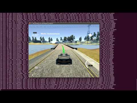
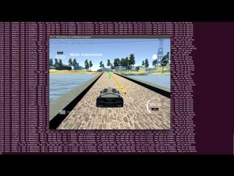
In this project, the aim is to implement a Model Predictive Controller (MPC) in C++. The controller is responsible for calculating the steering angle and the throttle value.
In order to implement MPC, the MPC class and the main.cpp file was modified. In addition, to change the parameters quickly the params class were added. In the MPC.cpp file, an instance of params class was created, and the required parameters were obtained from that instance.
Global Kinematic Model was used as described in the lessons. The position of the vehicle represented by x and y values. The angle which represents the car is shown by the psi value. Furthermore, the car has a velocity value. In addition, there is a cross track error (cte) value and the error on the psi value. The model aims to predict the next values of these variables using the actuations. The actuations consist of the delta value, steering angle in the project, and the acceleration value, throttle in the project. To represent the road, waypoints are provided from the simulator. A third order polynomial, which was constructed in main.cpp, represents the waypoints.
The velocity according to x-axis is calculated by multiplying the velocity (v0) and the cosine of the psi. Similarly, the velocity according to y-axis is calculated by multiplying the velocity and the sine of the psi value. Therefore, the x value at the next step is calculated with the summation of the previous x value and the velocity according to x-axis times the duration (dt). The y value at the next time step is calculated in the same way.
x1 = x0 + v0 * cos(psi0) * dt
y1 = y0 + v0 * sin(psi0) * dt
The psi value increases with the velocity (v) times steering angle value (delta) times the duration (dt) divided by the Lf value. The Lf value is the distance between the front of the vehicle and its center of gravity.
psi1 = psi0 + v0 * delta0 * dt / Lf
The velocity increased by the acceleration times duration.
v1 = v0 + a0 * dt
The cte error is calculated by the summation of the previous cte error and the velocity times sine of the epsi error times the duration. The previous cte error can be represented as the difference between current y value and the calculated y value from the third order polynomial (f0).
cte1 = (f0 - y0) + (v0 * sin(epsi0) * dt)
The epsi error is calculated by the current difference between the psi angle and the calculated angle using the arc tangent of the slope (m0) of the polynomial at x0. And adding the velocity times delta times duration divided by the Lf value.
epsi1 = (psi0 - arctan(m0)) + v0 + delta0 * dt / Lf
The actuations, the steering angle (delta), and the acceleration (a) were required to be determined in order to enable the car to drive on the track.
In the main.cpp, when data received from the simulator, the location of the car in 100ms future was predicted. The new x, y, psi, and v values are calculated according to the Global Kinematic Model. The steering value was used as delta, and the throttle value was used as acceleration. These values were obtained from the simulator. Then, main.cpp calculates the cte and the epsi values.
After predicting the future position of the vehicle, the points data were converted to vehicle coordinates, then transformed to vectors. The transformed points data was fit into a third order polynomial.
Selected N and dt values are 10 and 0.1 respectively. As in the previous work increasing the N value risks to obtain an optimum solution from the solver, and did not help with obtaining faster or smoother driving. Decreasing the N, worsen the turns on the curves. Changing the dt value as in the previous work to enable turns in advance did not help with the corrected model. In addition, increasing or decreasing the dt value did not provide improved results.
Target velocity was set to 55 m/s (123 MPH). Single target velocity was enough to drive safely.
To penalize higher cte, two addition cte_limits used. One of them was 1.5 and the other was 3.0. Two dummy variables introduced for every cte value. Their upperbounds were set to 1.5, and 3.0 respectively, and their lowerbounds were set to -1.5, and -3.0. Since the solver tries to minimize the total cost, if the cte value was between -1.5 and 1.5, the first dummy cte variable would be equal to the cte value, and the additional cost for that cte limit would be zero. On the other hand, if cte value is greater than 1.5 or less than -1.5, the dummy cte variable would be set to 1.5 or -1.5. As a result, the difference between the absolute value of the cte value and 1.5 would be squared and added to total cost. The cte limit with between -3.0 and 3.0, was added to the total cost in the same way.
The cost from the cte value, epsi value and the difference between reference velocity and the current velocity were also added to the total cost.
The cost from the steering angle value, and the difference in the steering angle value at the following time steps were added to the total cost. However, in the last model, the costs for the acceleration value are omitted.
There was an additional cost to provide in advance turns. The slope of the polynomial at the second time step is calculated, then it is multiplied with a variable (c_cte_mm1), then the difference between the current cte value and this value added to total cost after taking the square.
The N parameter was selected as 10. Increasing N caused longer solution times and did not provide better results. Decreasing N resulted in poor results. The dt was selected as 0.1 in the beginning. Then, to activate actuators in advance it was increased to 0.17. This enabled completing the track with higher speeds.
In order to have higher speed at straight sections and lower speed at sections with curve, the reference velocity was calculated as a function of the cte value. Other alternative tested were calculating the reference velocity as a function of the slope of the polynomial at the cars location. Using cte had better results.
To drive faster, the costs from actuations are omitted. Costs from cte, epsi, and velocity were used.
To penalize higher cte, two addition cte_limits used. One of them was 2.0 and the other was 3.5. Two dummy variables introduced for every cte value. Their upperbounds were set to 2.0, and 3.5 respectively, and their lowerbounds were set to -2.0, and -3.5. Since the solver tries to minimize the total cost, if the cte value was between -2.0 and 2.0, the first dummy cte variable would be equal to the cte value, and the additional cost for that cte limit would be zero. On the other hand, if cte value is greater than 2.0 or less than -2.0, the dummy cte variable would be set to 2.0 or -2.0. As a result, the difference between the absolute value of the cte value and 2.0 would be squared and added to total cost. The cte limit with between -3.5 and 3.5, was added to the total cost in the same way.
fg[0] += ((10 - t) / 5.5) * c_cte_l * CppAD::pow(vars[cte_start+t] - vars[cte_cor_start+t],2);
fg[0] += ((10 - t) / 5.5) * c_cte_l2 * CppAD::pow(vars[cte_start+t] - vars[cte_cor_start2+t],2);
In order to increase the importance of the actuations in the first steps, a multiplier added to the cte limit costs. The cost of the first step was multiplied by 10, the cost of the second step was multiplied by 9, and so on. Then these costs were divided by 5.5, which is the average value of the multipliers for ten steps (10, 9, 8, 7, 6, 5, 4, 3, 2, 1). This multiplier enabled driving at higher speeds.
The cost from the cte value, epsi value and the difference between reference velocity and the current velocity were also added to the total cost.
      fg[0] += c_cte * CppAD::pow(vars[cte_start+t],2);
      fg[0] += c_epsi * CppAD::pow(vars[epsi_start+t],2);
      fg[0] += c_v * CppAD::pow(vars[v_start+t] - ref_v,2);
In order to supply appropriate values for actuations, the actuations for the first step were set to zero, and the actuations for the second step were sent to the simulator. Since was dt = 0.1 and delay was 0.1 seconds, the actuations of the second step were able to drive the track. However, the car started turning as the curve began or after the curve began. In order to make the car start turning in advance, the dt value was increased to 0.17. This enabled the car to go faster.
- cmake >= 3.5
- make >= 4.1
- gcc/g++ >= 5.4
- uWebSockets
- Fortran Compiler
- Ipopt
- CppAD
- Eigen.
- Clone this repo.
- Make a build directory:
mkdir build && cd build - Compile:
cmake .. && make - Run it:
./mpc.
