Probability (chances/ likelihood/ likeliness)

Probability is chance of event happening. In other words, what are the chances that we might expect a particular outcome from an experiment. Mathematically, It a number between [0, 1] which tells, "how likely it is that we may expect a particular outcome".

Dependent And Independent Event

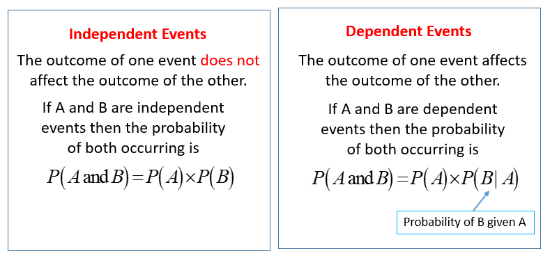
Dependent events are events that affect each other. Outcome of one event has direct affect to outcome of other event and so if event A changes, It will change likelihood of event B and vice-versa(imagine drawing a ball from a jug containing different colour balls without replacement).

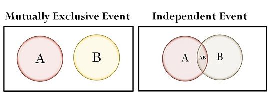
Independent events are the events where outcome of one event has no affect on outcome of other (imagine tossing a coin or rolling a dice multiple times).

Independent event vs mutually exclusive

For Independent events Probability of P(A and B) = P(A) * P(B)
For Independent events Probability of P(A|B) = P(A)
For mutually exclusive events P(A and B) = 0
For mutually exclusive events P(A|B) = 0

Conditional Probability

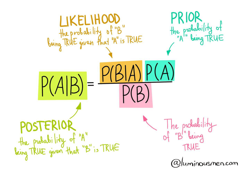
Conditional probability is probability of event happening, Given a certain event has already occurred. Here both event A and event B should be dependent (their intersection must not be 0). Otherwise P(A|B) = P(A).

Marginal, Joint, And Conditional Probability

Marginal Probability: The probability of an event irrespective of the outcomes of other random variables, e.g. P(A).

The joint probability is the probability of two (or more) simultaneous events, often described in terms of events A and B from two dependent random variables, e.g. X and Y. The joint probability is often summarized as just the outcomes, e.g. A and B.

Joint Probability: Probability of two (or more) simultaneous events, e.g. P(A and B) or P(A, B).

The conditional probability is the probability of one event given the occurrence of another event, often described in terms of events A and B from two dependent random variables e.g. X and Y.

Conditional Probability: Probability of one (or more) event given the occurrence of another event, e.g. P(A given B) or P(A | B)

The joint probability can be calculated using the conditional probability; for example:

P(A, B) = P(A | B) * P(B)

This is called the product rule. Importantly, the joint probability is symmetrical, meaning that:

P(A, B) = P(B, A)

The conditional probability can be calculated using the joint probability; for example:

P(A | B) = P(A, B) / P(B)

The conditional probability is not symmetrical; for example:

P(A | B) != P(B | A)

From conditional probability to bayes theorem

Bayes theorem(a way of finding conditional probability)

Bayes theorem describes the probability of an event based on the prior knowledge of conditions that might be related to the events. Posterior = (Likelihood * Prior) / Evidence

Here is how Bayes theorem expression look like

Probability vs Likelihood(in the context of distribution of continuous variable)

While probability value is the area under the curve which gives a value between[0, 1] telling how probable it is that a value would fall between the given range (lets say between 50-100), where else likelihood is the point on curve which tells, given the distribution what is the probability of observing a point within the distribution.

* Note probability of a point is zero (because there is no area of line)

StatQuest, probability vs likelihood

StatQuest: Probability vs Likelihood

Naïve Bayes (probabilistic classification algorithm)

Naïve Bayes is a classification algorithm (probabilistic classifier) with naïve assumption that features are conditional independent (or independent) of each other. This is naïve because in real world, feature are not really dependent (they depend on each other and other affect the target variable).

Naïve Bayes uses Bayes theorem to compute probability of x_i belongs to class label y_i. Naïve Bayes makes this assumption to simplify calculations unlike Bayesian belief network, which tries to model conditional dependence.

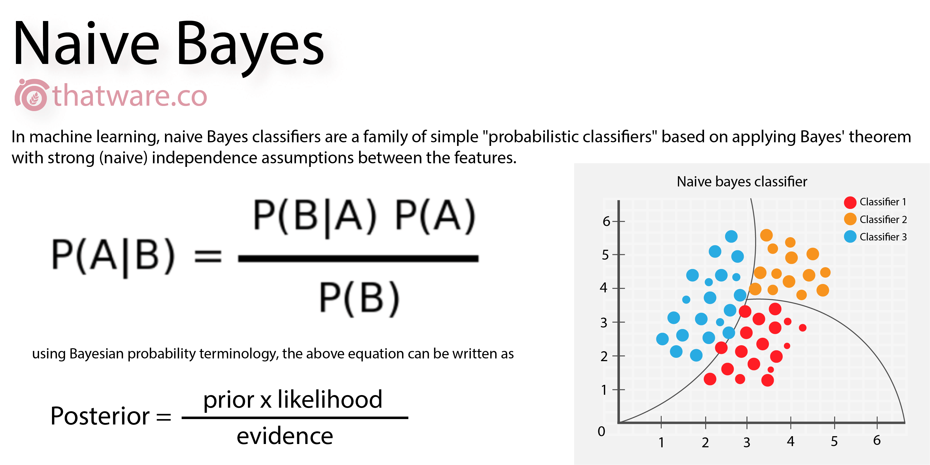
Assumption of Naïve Bayes algorithm

Naïve Bayes assumes that are features are conditional independent of each other, It makes this assumption to make computations much simpler
It also assumes classes are balanced because probabilities given by Naïve Bayes will be highly skewed towards majority class.

Mathematics formulation of naïve Bayes

Formulation is simple, if you follow Bayes theorem, it's just a chain rule. For each give class, we compute probability of a class given the data point, which is P(C_k| f1 & f2 & f3). If you notice here, we are searching for exact x which has f1, f2, f3 values. For instance, if f1=0.009, f2= 12, f3= "cyan" finding the rows with exact match would be really low, this is where our naïve Bayes could fail miserably.

Also notice, we remove the denominator because it is constant for all the class, so it doesn't matter, because all the numerator value would be relatively hold true for most of the expect. For instance:

take 12/4 and 15/4, we know 15>12 so is 3.75(15/4) > 3(12/4) So the relative value is preserved even though values itself has been changed.

Naïve Bayes without conditional independence

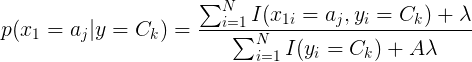
To make naïve Bayes work, we make current feature independent to other features, for instance

For f1 the expression P(C_k| f1 & f2 & f3) = P(C_k| f1). As you can our assumption in action. We do this for all features and lastly multiply the expression with the prior probability of the corresponding class (which is just the count of occurrence of class K divided by the number of rows in the train set).

Naïve Bayes with conditional independence.

Maximum A posterior (MAP) estimation (choosing class which yields maximum posterior probability)

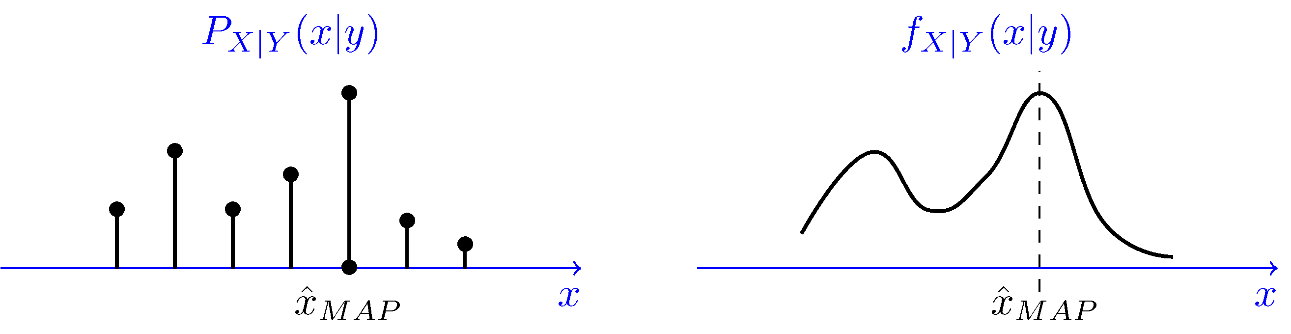
MAP of X given Y, X|Y = y is the value of x that maximizes posterior PDF or PMF. The MAP estimate of X is usually shown by x_hat MAP.

To predict a class, NB uses MAP, which yields class that has maximum probability.

Naïve Bayes in a nutshell

Here is how to compute prior(class probabilities) and conditional probabilities (class-feature pair probabilities)

Computing probabilities in Naïve Bayes

Additive smoothing and Log of probabilities (performing additional operations to solve some challenges in naïve Bayes)

**Additive smoothing/ Laplace smoothing: ** is to resolve the problem of 0 probability. If a feature/ word is not present in train data but in test data, then setting P(w'| y=1) = 1 could confuse the algorithm. If we set P(w'| y=1) = 0 then whole probability will be 0, multiplying any number with 0 is 0. To get around with this problem we add a constant alpha in numerator and alpha * K in denominator where K is the count of distinct item in a feature or it could also be number of features.

Class-feature pair probabilities with additive smoothing

If alpha is large, we make probability distribution close to uniform distribution (under fitting, If alpha is small, we tend to overfit

*Note: Alpha is related to bias-variance trade off

Laplace smoothing in Naïve Bayes algorithm

Log of probabilities: we log probabilities because log is a monotonic function (strictly increasing or decreasing). Taking log of probabilities solves the problem of huge floating number (computer might round it for it's convenience with might mess up with class probability). Multiplying smaller number with smaller number results in even more smaller number.

Log also has a property of converting multiplication into addition log(a * b) = log(a) + log(b)), Also, we use log probabilities if data has large dimension, as to multiplying numbers between 0 and 1 many time could result in round offs by python.

15. Floating Point Arithmetic: Issues and Limitations

Handling continuous data

Continuous data is handled by making assumption about the distribution of data. In other words, if we compute likelihood from gaussian distribution, It is called gaussian naïve Bayes, if we compute likelihood from binomial distribution,It is called Bernoulli naïve Bayes and so on.

We compute statistics based on the distribution. If we choose gaussian distribution (gaussian naïve Bayes) we compute mean and standard deviation class-feature wise, which later will be used to compute likelihood for query point.

Trained data: computing statistics

Test data example

Test data: computing likelihood based on the statistics computed on train data

Computing actual probabilities class-wise

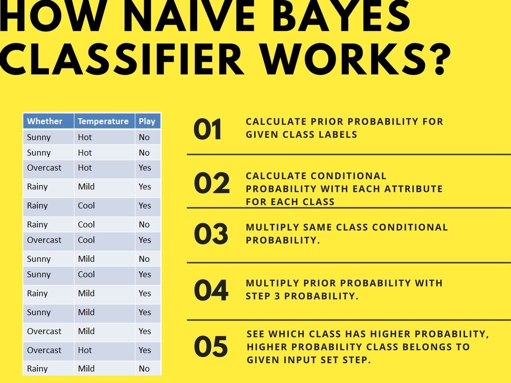
Use Naive Bayes Algorithm for Categorical and Numerical data classification

KEY TAKEAWAYS

Assumes Conditional independence: One of the big assumptions in naïve Bayes is that, features are independent of each other given the class label.
Simple to compute : In naïve Bayes, Only stored probability needs to be multiplied (or added in the case of log probability) which doesn't require huge computation.
Simple to store: We just need to store probabilities of each value in each feature for each pass. Which takes roughly ( d * c), where d is the number of features and c is the number of classes.
Works fairly well even if some features are not independent .
Uses Laplace smoothing (Additive smoothing) so that probability of seeing unseen data attribute don't become 0.
Uses log of probabilities to get around with problem of numerical instability . Imagine multiplying lots of number smaller than 0 (resulting number will be even more smaller).
Can be used as baseline model as it is fast to train, and less parameters to be tuned. A baseline is a model whose results can be used to compare results of other advance models.
Naïve Bayes is one of popular methods to solve text categorization problem, the problem of judging documents as belonging to one category or the other, such as email spam detection.
Using log of probabilities if dimension of data is too high.
Deals with outlier easily.
Prone to imbalanced class distribution, as majority class prior will have more weight and hence can influence overall probability value.
Although naïve Bayes is known as a decent classifier, it is known to be a bad estimator, so the probability outputs from predict_proba are not to be taken too seriously.
Feature importance is easy to get in the case of NB, For each feature and for each value in a feature, for each class, we declare best feature value that has huge contributions towards decision making. Hence we choose feature value that has maximum probability given for a class.
Naïve Bayes models are a group of extremely fast and simple classification algorithms that are often suitable for very high-dimensional datasets. Because they are so fast and have so few tuneable parameters, they end up being very useful as a quick-and-dirty baseline for a classification problem.
NB is not robust to imbalanced class distribution, as majority class priors will be higher than than the minority class, this gives unfair advantage to majority class to influence class predictions.

Another Affect of class imbalance is, Alpha will have more impact on minority class than on majority class, As minority class will have less value in denominator the overall ratio will be more compared to majority class.

To get around the problem of class imbalance we may use few technique,
1. Up sampling minority class or Down sampling majority class, we may also use class weights to compensate for class imbalance.
2. Dropping prior probabilities, as we have know, we multiply priors which are P(y=class_label), we could just drop this expression as this would be huge for majority class which would skew the prediction towards majority class.
Bias variance trade-off is controlled by alpha parameter (which is Laplace smoothing/ additive smoothing).

Low value of alpha results in overfitting.

High value of alpha results in underfitting, as it pushes probability of feature values/ word towards uniform distribution and hence there is nothing much to learn from the data which has same value. It all boils down to prior classes, which is

p(1) = # of class 0 instance/ total number of points

p(2) = # of class 1 instance/ total number of instance

so, prediction of our model will be biased towards the majority class, just like in KNN classifier