malmgrek / gammy

:octopus: Generalized additive models in Python with a Bayesian twist

Gammy – Generalized additive models in Python with a Bayesian twist

A Generalized additive model is a predictive mathematical model defined as a sum of terms that are calibrated (fitted) with observation data.

Generalized additive models form a surprisingly general framework for building models for both production software and scientific research. This Python package offers tools for building the model terms as decompositions of various basis functions. It is possible to model the terms e.g. as Gaussian processes (with reduced dimensionality) of various kernels, as piecewise linear functions, and as B-splines, among others. Of course, very simple terms like lines and constants are also supported (these are just very simple basis functions).

The uncertainty in the weight parameter distributions is modeled using Bayesian statistical analysis with the help of the superb package BayesPy. Alternatively, it is possible to fit models using just NumPy.

Table of Contents

• Installation
• Examples
  • Polynomial regression on 'roids
    • Predicting with model
    • Plotting results
    • Saving model on hard disk
  • Gaussian process regression
    • More covariance kernels
    • Defining custom kernels
  • Spline regression
  • Non-linear manifold regression
• Testing
• Package documentation

Installation

The package is found in PyPi.

pip install gammy

Examples

In this overview, we demonstrate the package's most important features through common usage examples.

Polynomial regression on 'roids

A typical simple (but sometimes non-trivial) modeling task is to estimate an unknown function from noisy data. First we import the bare minimum dependencies to be used in the below examples:

>>> import numpy as np

>>> import gammy
>>> from gammy.models.bayespy import GAM

>>> gammy.__version__
'0.5.5'

Let's simulate a dataset:

>>> np.random.seed(42)

>>> n = 30
>>> input_data = 10 * np.random.rand(n)
>>> y = 5 * input_data + 2.0 * input_data ** 2 + 7 + 10 * np.random.randn(n)

The object x is just a convenience tool for defining input data maps as if they were just Numpy arrays:

>>> from gammy.arraymapper import x

Define and fit the model:

>>> a = gammy.formulae.Scalar(prior=(0, 1e-6))
>>> b = gammy.formulae.Scalar(prior=(0, 1e-6))
>>> bias = gammy.formulae.Scalar(prior=(0, 1e-6))
>>> formula = a * x + b * x ** 2 + bias
>>> model = GAM(formula).fit(input_data, y)

The model attribute model.theta characterizes the Gaussian posterior distribution of the model parameters vector.

>>> model.mean_theta
[array([3.20130444]), array([2.0420961]), array([11.93437195])]

Variance of additive zero-mean normally distributed noise is estimated automagically:

>>> round(model.inv_mean_tau, 8)
74.51660744

Predicting with model

>>> model.predict(input_data[:2])
array([ 52.57112684, 226.9460579 ])

Predictions with uncertainty, that is, posterior predictive mean and variance can be calculated as follows:

>>> model.predict_variance(input_data[:2])
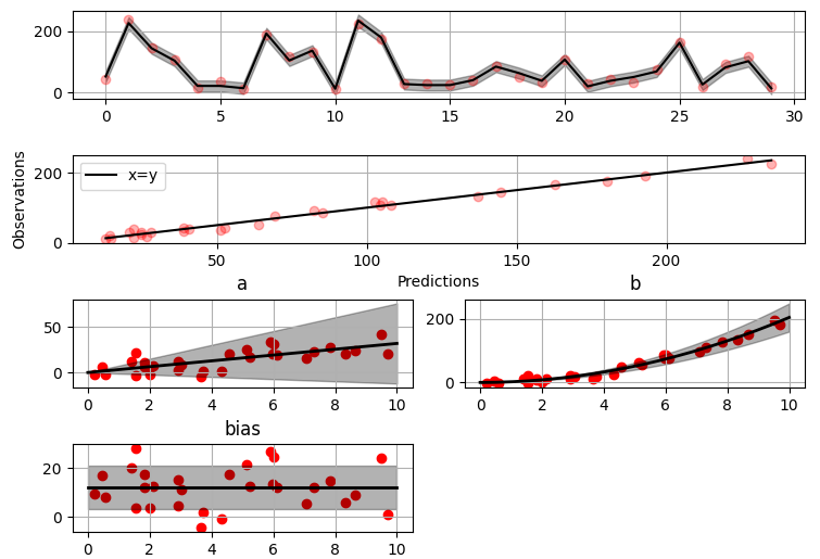
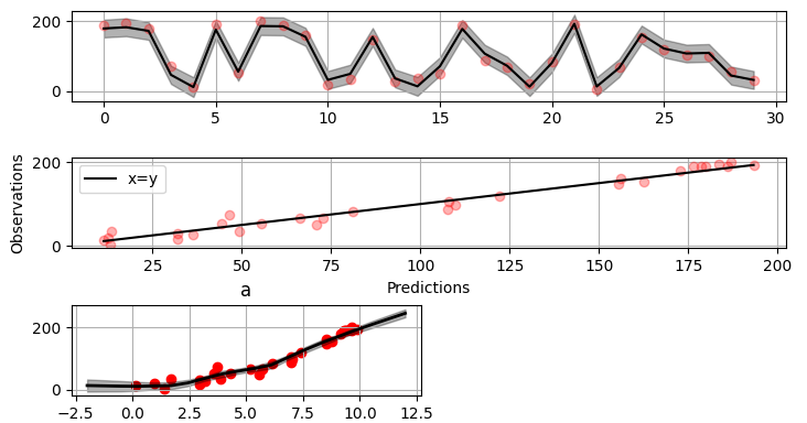
(array([ 52.57112684, 226.9460579 ]), array([79.35827362, 95.16358131]))

Plotting results

>>> fig = gammy.plot.validation_plot(
...     model,
...     input_data,
...     y,
...     grid_limits=[0, 10],
...     input_maps=[x, x, x],
...     titles=["a", "b", "bias"]
... )

The grey band in the top figure is two times the prediction standard deviation and, in the partial residual plots, two times the respective marginal posterior standard deviation.

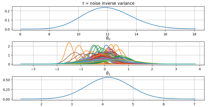
It is also possible to plot the estimated Γ-distribution of the noise precision (inverse variance) as well as the 1-D Normal distributions of each individual model parameter.

Plot (prior or posterior) probability density functions of all model parameters:

>>> fig = gammy.plot.gaussian1d_density_plot(model)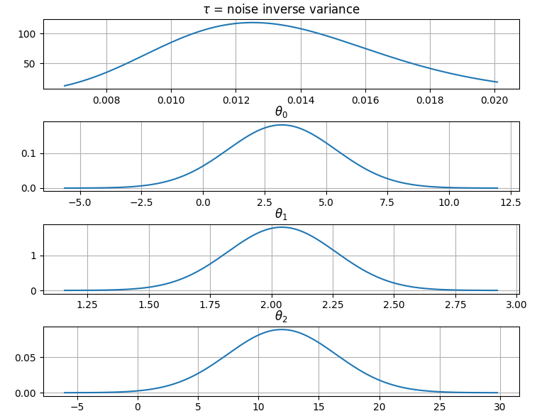

Saving model on hard disk

Saving:

>> model.save("/home/foobar/test.hdf5")

Loading:

>> model = GAM(formula).load("/home/foobar/test.hdf5")

Gaussian process regression

Create fake dataset:

>>> n = 50
>>> input_data = np.vstack((2 * np.pi * np.random.rand(n), np.random.rand(n))).T
>>> y = (
...     np.abs(np.cos(input_data[:, 0])) * input_data[:, 1] +
...     1 + 0.1 * np.random.randn(n)
... )

Define model:

>>> a = gammy.formulae.ExpSineSquared1d(
...     np.arange(0, 2 * np.pi, 0.1),
...     corrlen=1.0,
...     sigma=1.0,
...     period=2 * np.pi,
...     energy=0.99
... )
>>> bias = gammy.Scalar(prior=(0, 1e-6))
>>> formula = a(x[:, 0]) * x[:, 1] + bias
>>> model = gammy.models.bayespy.GAM(formula).fit(input_data, y)

>>> round(model.mean_theta[0][0], 8)
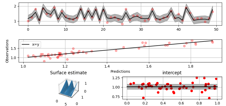
-0.8343458

Plot predictions and partial residuals:

>>> fig = gammy.plot.validation_plot(
...     model,
...     input_data,
...     y,
...     grid_limits=[[0, 2 * np.pi], [0, 1]],
...     input_maps=[x[:, 0:2], x[:, 1]],
...     titles=["Surface estimate", "intercept"]
... )

Plot parameter probability density functions

>>> fig = gammy.plot.gaussian1d_density_plot(model)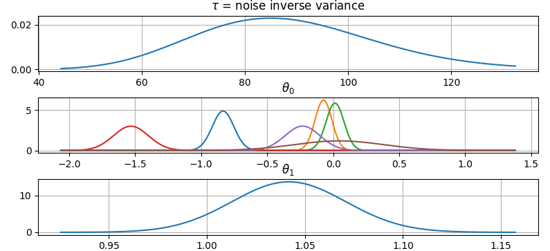

More covariance kernels

The package contains covariance functions for many well-known options such as the Exponential squared, Periodic exponential squared, Rational quadratic, and the Ornstein-Uhlenbeck kernels. Please see the documentation section More on Gaussian Process kernels for a gallery of kernels.

Defining custom kernels

Please read the documentation section: Customize Gaussian Process kernels

Spline regression

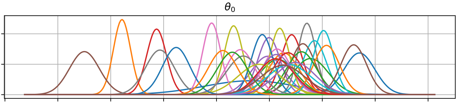
Constructing B-Spline based 1-D basis functions is also supported. Let's define dummy data:

>>> n = 30
>>> input_data = 10 * np.random.rand(n)
>>> y = 2.0 * input_data ** 2 + 7 + 10 * np.random.randn(n)

Define model:

>>> grid = np.arange(0, 11, 2.0)
>>> order = 2
>>> N = len(grid) + order - 2
>>> sigma = 10 ** 2
>>> formula = gammy.BSpline1d(
...     grid,
...     order=order,
...     prior=(np.zeros(N), np.identity(N) / sigma),
...     extrapolate=True
... )(x)
>>> model = gammy.models.bayespy.GAM(formula).fit(input_data, y)

>>> round(model.mean_theta[0][0], 8)
-49.00019115

Plot validation figure:

>>> fig = gammy.plot.validation_plot(
...     model,
...     input_data,
...     y,
...     grid_limits=[-2, 12],
...     input_maps=[x],
...     titles=["a"]
... )

Plot parameter probability densities:

>>> fig = gammy.plot.gaussian1d_density_plot(model)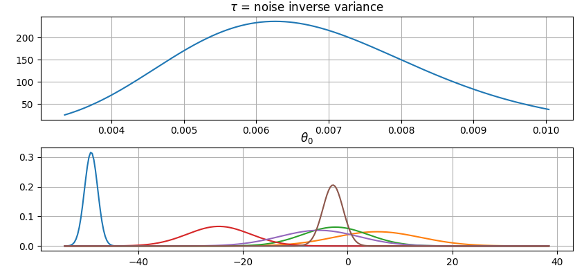

Non-linear manifold regression

In this example we try estimating the bivariate "MATLAB function" using a Gaussian process model with Kronecker tensor structure (see e.g. PyMC3). The main point in the below example is that it is quite straightforward to build models that can learn arbitrary 2D-surfaces.

Let us first create some artificial data using the MATLAB function!

>>> n = 100
>>> input_data = np.vstack((
...     6 * np.random.rand(n) - 3, 6 * np.random.rand(n) - 3
... )).T
>>> y = (
...     gammy.utils.peaks(input_data[:, 0], input_data[:, 1]) +
...     4 + 0.3 * np.random.randn(n)
... )

There is support for forming two-dimensional basis functions given two one-dimensional formulas. The new combined basis is essentially the outer product of the given bases. The underlying weight prior distribution priors and covariances are constructed using the Kronecker product.

>>> a = gammy.ExpSquared1d(
...     np.arange(-3, 3, 0.1),
...     corrlen=0.5,
...     sigma=4.0,
...     energy=0.99
... )(x[:, 0])  # NOTE: Input map is defined here!
>>> b = gammy.ExpSquared1d(
...     np.arange(-3, 3, 0.1),
...     corrlen=0.5,
...     sigma=4.0,
...     energy=0.99
... )(x[:, 1]) # NOTE: Input map is defined here!
>>> A = gammy.formulae.Kron(a, b)
>>> bias = gammy.formulae.Scalar(prior=(0, 1e-6))
>>> formula = A + bias
>>> model = GAM(formula).fit(input_data, y)

>>> round(model.mean_theta[0][0], 8)
0.37426986

Note that same logic could be used to construct higher dimensional bases, that is, one could define a 3D-formula:

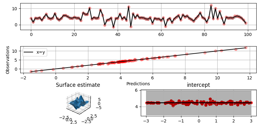
>> formula_3d = gammy.Kron(gammy.Kron(a, b), c)

Plot predictions and partial residuals:

>>> fig = gammy.plot.validation_plot(
...     model,
...     input_data,
...     y,
...     grid_limits=[[-3, 3], [-3, 3]],
...     input_maps=[x, x[:, 0]],
...     titles=["Surface estimate", "intercept"]
... )

Plot parameter probability density functions:

>>> fig = gammy.plot.gaussian1d_density_plot(model)

Testing

The package's unit tests can be ran with PyTest (cd to repository root):

pytest -v

Running this documentation as a Doctest:

python -m doctest -v README.md

Package documentation

Documentation of the package with code examples: https://malmgrek.github.io/gammy.

gammy's Issues

How do you fit more than one feature?

Tweedie distribution

Is there a way to fit a gam with a Tweedie distribution?

A Tweedie distribution is a mixture between a poison and a gamma distribution. It helps model insurance losses with a significant positive probability mass at 0 (because most customers do not claim losses).

Taking energy>1 in covariance kernels fails

Sometimes one would like to use the full basis in the computation (e.g. some illustration) and not use the dimension reduction trick. Setting energy > 1 should give you all the basis functions, but this fails, since some of the eigenvalues returned by np.linalg.eigh are negative for some reason (very small negative numbers). Using np.linalg.svd instead would solve the issue.

Doubt regarding kron() function

Hello, thank you for this wonderful library. I stumbled upon the kron() function while exploring it. Could you please clarify whether this function is exactly the same as the tensor smooth product as provided in mgcv package of R.