Coder Social home page Coder Social logo

lieberinstitute / spatialdlpfc Goto Github PK

View Code? Open in Web Editor NEW
10.0 9.0 0.0 15.23 GB

spatialDLPFC project involving Visium (n = 30), Visium SPG (n = 4) and snRNA-seq (n = 19) samples

Home Page: http://research.libd.org/spatialDLPFC/

R 0.31% Shell 0.05% HTML 98.66% MATLAB 0.01% Python 0.09% Jupyter Notebook 0.88%
rstats visium dlpfc transcriptomics bioconductor spatialdlpfc visium-spg spatial-transcriptomics

spatialdlpfc's Introduction

spatialDLPFC

DOI

Overview

Welcome to the spatialDLPFC project! This project involves 3 data types as well as several interactive websites, all of which you are publicly accessible for you to browse and download.

In this project we studied spatially resolved and single nucleus transcriptomics data from the dorsolateral prefrontal cortex (DLPFC) from postmortem human brain samples. From 10 neurotypical controls we generated spatially-resolved transcriptomics data using using 10x Genomics Visium across the anterior, middle, and posterior DLPFC (n = 30). We also generated single nucleus RNA-seq (snRNA-seq) data using 10x Genomics Chromium from 19 of these tissue blocks. We further generated data from 4 adjacent tissue slices with 10x Genomics Visium Spatial Proteogenomics (SPG), that can be used to benchmark spot deconvolution algorithms. This work is being was performed by the Keri Martinowich, Leonardo Collado-Torres, and Kristen Maynard teams at the Lieber Institute for Brain Development as well as Stephanie Hicks’s group from JHBSPH’s Biostatistics Department.

This project involves the GitHub repositories LieberInstitute/spatialDLPFC and LieberInstitute/DLPFC_snRNAseq.

If you tweet about this website, the data or the R package please use the #spatialDLPFC hashtag. You can find previous tweets that way as shown here.

Thank you for your interest in our work!

Study Design

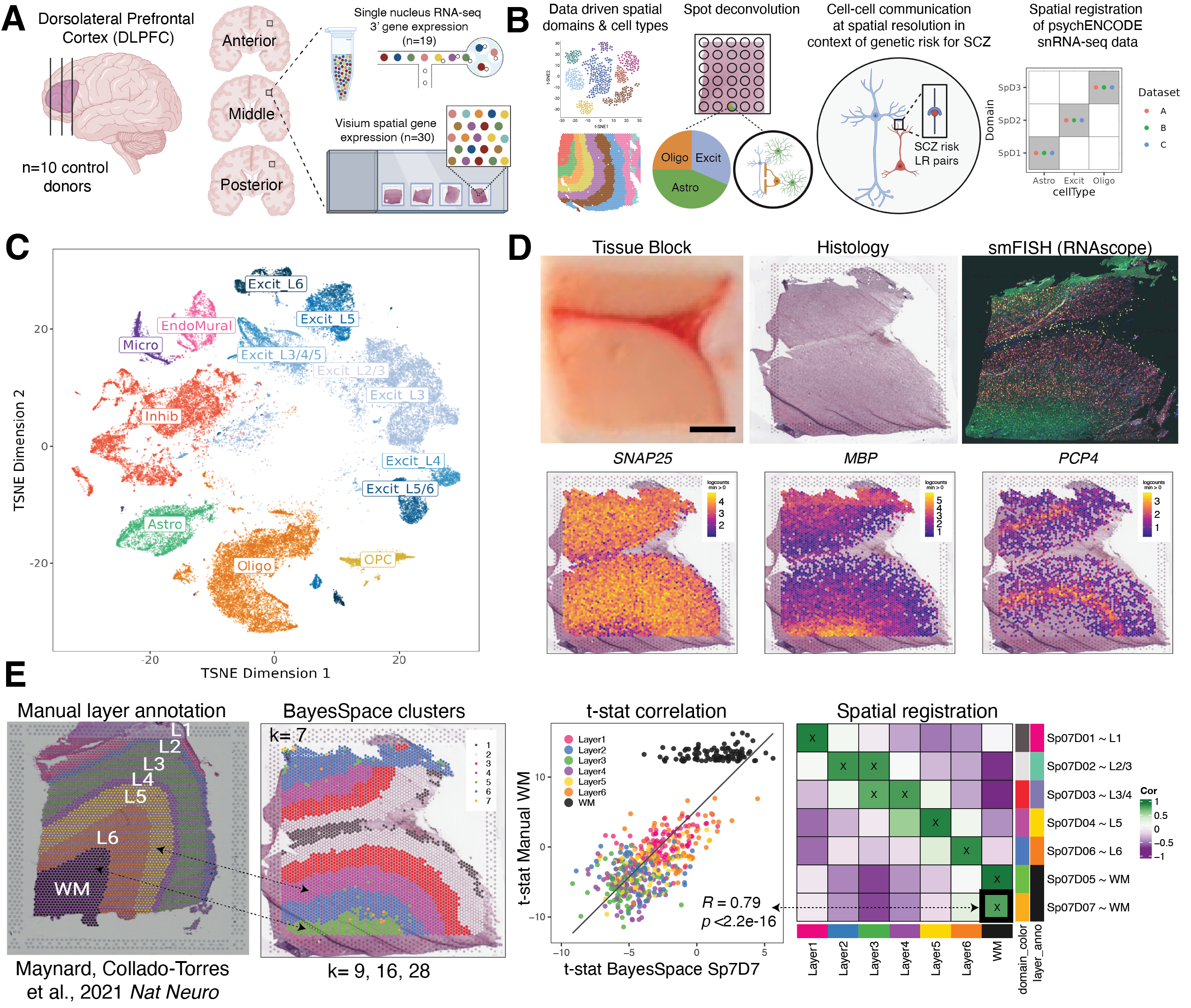
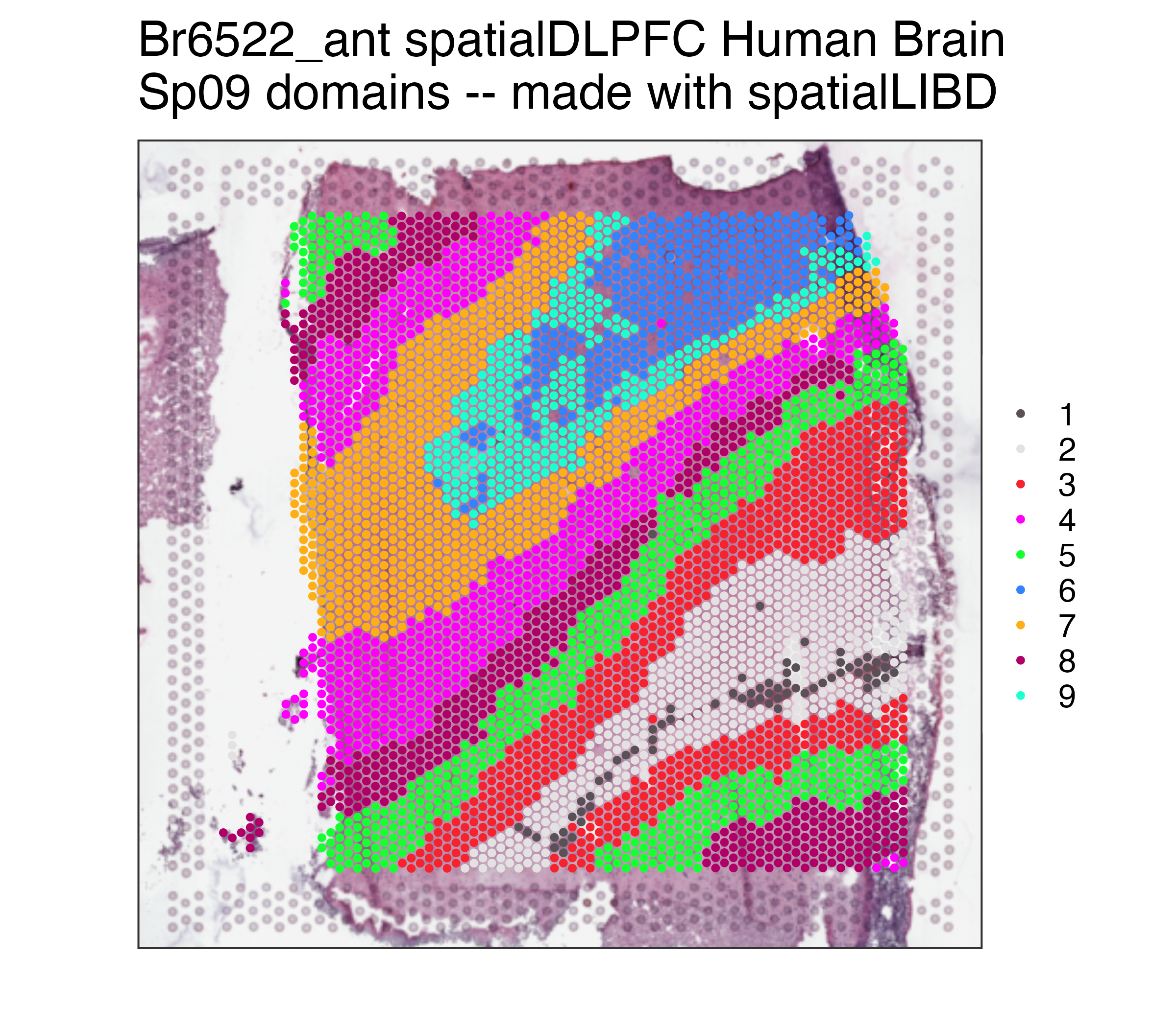
Study design to generate paired single nucleus RNA-sequencing (snRNA-seq) and spatially-resolved transcriptomic data across DLPFC. (A) DLPFC tissue blocks were dissected across the rostral-caudal axis from 10 adult neurotypical control postmortem human brains, including anterior (Ant), middle (Mid), and posterior (Post) positions (n=3 blocks per donor, n=30 blocks total). The same tissue blocks were used for snRNA-seq (10x Genomics 3’ gene expression assay, n=1-2 blocks per donor, n=19 samples) and spatial transcriptomics (10x Genomics Visium spatial gene expression assay, n=3 blocks per donor, n=30 samples). (B) Paired snRNA-seq and Visium data were used to identify data-driven spatial domains (SpDs) and cell types, perform spot deconvolution, conduct cell-cell communication analyses, and spatially register companion PsychENCODE snRNA-seq DLPFC data. (C) t-distributed stochastic neighbor embedding (t-SNE) summarizing layer resolution cell types identified by snRNA-seq. (D) Tissue block orientation and morphology was confirmed by hematoxylin and eosin (H&E) staining and single molecule fluorescent in situ hybridization (smFISH) with RNAscope (SLC17A7 marking excitatory neurons in pink, MBP marking white matter (WM) in green, RELN marking layer (L)1 in yellow, and NR4A2 marking L6 in orange). Scale bar is 2mm. Spotplots depicting log transformed normalized expression (logcounts) of SNAP25, MBP, and PCP4 in the Visium data confirm the presence of gray matter, WM, and cortical layers, respectively. (E) Schematic of unsupervised SpD identification and registration using BayesSpace SpDs at k=7. Enrichment t-statistics computed on BayesSpace SpDs were correlated with manual histological layer annotations from (Maynard, Collado-Torres et al., 2021, Nat Neuro) to map SpDs to known histological layers. The heatmap of correlation values summarizes the relationship between BayesSpace SpDs and classic histological layers. Higher confidence annotations (⍴ > 0.25, merge ratio = 0.1) are marked with an “X”.

Interactive Websites

All of these interactive websites are powered by open source software, namely:

We provide the following interactive websites, organized by dataset with software labeled by emojis:

Local spatialLIBD apps

If you are interested in running the spatialLIBD applications locally, you can do so thanks to the spatialLIBD::run_app(), which you can also use with your own data as shown in our vignette for publicly available datasets provided by 10x Genomics.

## Run this web application locally with:
spatialLIBD::run_app()

## You will have more control about the length of the session and memory usage.
## See http://research.libd.org/spatialLIBD/reference/run_app.html#examples
## for the full R code to run https://libd.shinyapps.io/spatialDLPFC_Visium_Sp09
## locally. See also:
## * https://github.com/LieberInstitute/spatialDLPFC/tree/main/code/deploy_app_k09
## * https://github.com/LieberInstitute/spatialDLPFC/tree/main/code/deploy_app_k09_position
## * https://github.com/LieberInstitute/spatialDLPFC/tree/main/code/deploy_app_k09_position_noWM
## * https://github.com/LieberInstitute/spatialDLPFC/tree/main/code/deploy_app_k16
## * https://github.com/LieberInstitute/spatialDLPFC/tree/main/code/analysis_IF/03_spatialLIBD_app

## You could also use spatialLIBD::run_app() to visualize your
## own data given some requirements described
## in detail in the package vignette documentation
## at http://research.libd.org/spatialLIBD/.

Contact

We value public questions, as they allow other users to learn from the answers. If you have any questions, please ask them at LieberInstitute/spatialDLPFC/issues and refrain from emailing us. Thank you again for your interest in our work!

Citing our work

Please cite this manuscript if you use data from this project.

Integrated single cell and unsupervised spatial transcriptomic analysis defines molecular anatomy of the human dorsolateral prefrontal cortex Louise A. Huuki-Myers, Abby Spangler, Nicholas J. Eagles, Kelsey D. Montgomery, Sang Ho Kwon, Boyi Guo, Melissa Grant-Peters, Heena R. Divecha, Madhavi Tippani, Chaichontat Sriworarat, Annie B. Nguyen, Prashanthi Ravichandran, Matthew N. Tran, Arta Seyedian, PsychENCODE Consortium, Thomas M. Hyde, Joel E. Kleinman, Alexis Battle, Stephanie C. Page, Mina Ryten, Stephanie C. Hicks, Keri Martinowich, Leonardo Collado-Torres, Kristen R. Maynard bioRxiv 2023.02.15.528722; doi: https://doi.org/10.1101/2023.02.15.528722

Below is the citation in BibTeX format.

@article {Huuki-Myers2023.02.15.528722,
    author = {Huuki-Myers, Louise A. and Spangler, Abby and Eagles, Nicholas J. and Montgomery, Kelsey D. and Kwon, Sang Ho and Guo, Boyi and Grant-Peters, Melissa and Divecha, Heena R. and Tippani, Madhavi and Sriworarat, Chaichontat and Nguyen, Annie B. and Ravichandran, Prashanthi and Tran, Matthew N. and Seyedian, Arta and , and Hyde, Thomas M. and Kleinman, Joel E. and Battle, Alexis and Page, Stephanie C. and Ryten, Mina and Hicks, Stephanie C. and Martinowich, Keri and Collado-Torres, Leonardo and Maynard, Kristen R.},
    title = {Integrated single cell and unsupervised spatial transcriptomic analysis defines molecular anatomy of the human dorsolateral prefrontal cortex},
    elocation-id = {2023.02.15.528722},
    year = {2023},
    doi = {10.1101/2023.02.15.528722},
    publisher = {Cold Spring Harbor Laboratory},
    URL = {https://www.biorxiv.org/content/early/2023/02/15/2023.02.15.528722},
    eprint = {https://www.biorxiv.org/content/early/2023/02/15/2023.02.15.528722.full.pdf},
    journal = {bioRxiv}
}

Cite spatialLIBD

Below is the citation output from using citation('spatialLIBD') in R. Please run this yourself to check for any updates on how to cite spatialLIBD.

print(citation("spatialLIBD")[1], bibtex = TRUE)
#> Pardo B, Spangler A, Weber LM, Hicks SC, Jaffe AE, Martinowich K,
#> Maynard KR, Collado-Torres L (2022). "spatialLIBD: an R/Bioconductor
#> package to visualize spatially-resolved transcriptomics data." _BMC
#> Genomics_. doi:10.1186/s12864-022-08601-w
#> <https://doi.org/10.1186/s12864-022-08601-w>,
#> <https://doi.org/10.1186/s12864-022-08601-w>.
#> 
#> A BibTeX entry for LaTeX users is
#> 
#>   @Article{,
#>     title = {spatialLIBD: an R/Bioconductor package to visualize spatially-resolved transcriptomics data},
#>     author = {Brenda Pardo and Abby Spangler and Lukas M. Weber and Stephanie C. Hicks and Andrew E. Jaffe and Keri Martinowich and Kristen R. Maynard and Leonardo Collado-Torres},
#>     year = {2022},
#>     journal = {BMC Genomics},
#>     doi = {10.1186/s12864-022-08601-w},
#>     url = {https://doi.org/10.1186/s12864-022-08601-w},
#>   }

Please note that the spatialLIBD was only made possible thanks to many other R and bioinformatics software authors, which are cited either in the vignettes and/or the paper(s) describing the package.

Cite Samui

To cite samui please use:

Performant web-based interactive visualization tool for spatially-resolved transcriptomics experiments Chaichontat Sriworarat, Annie Nguyen, Nicholas J. Eagles, Leonardo Collado-Torres, Keri Martinowich, Kristen R. Maynard, Stephanie C. Hicks Biological Imaging; doi: https://doi.org/10.1017/S2633903X2300017X

Below is the citation in BibTeX format.

@article{sriworarat_performant_2023,
    title = {Performant web-based interactive visualization tool for spatially-resolved transcriptomics experiments},
    volume = {3},
    issn = {2633-903X},
    url = {https://www.cambridge.org/core/journals/biological-imaging/article/performant-webbased-interactive-visualization-tool-for-spatiallyresolved-transcriptomics-experiments/B66303984D10B9E5A23D3656CB8537C0},
    doi = {10.1017/S2633903X2300017X},
    language = {en},
    urldate = {2024-04-19},
    journal = {Biological Imaging},
    author = {Sriworarat, Chaichontat and Nguyen, Annie and Eagles, Nicholas J. and Collado-Torres, Leonardo and Martinowich, Keri and Maynard, Kristen R. and Hicks, Stephanie C.},
    month = jan,
    year = {2023},
    keywords = {georeferencing, interactive image viewer, multi-dimensional image, single-cell transcriptomics, spatially resolved transcriptomics, web-based browser},
    pages = {e15}
}

Cite VistoSeg

To cite VistoSeg please use:

VistoSeg: {Processing utilities for high-resolution images for spatially resolved transcriptomics data. Madhavi Tippani, Heena R. Divecha, Joseph L. Catallini II, Sang Ho Kwon, Lukas M. Weber, Abby Spangler, Andrew E. Jaffe, Thomas M. Hyde, Joel E. Kleinman, Stephanie C. Hicks, Keri Martinowich, Leonardo Collado-Torres, Stephanie C. Page, Kristen R. Maynard Biological Imaging ; doi: https://doi.org/10.1017/S2633903X23000235

Below is the citation in BibTeX format.

@article{tippani_vistoseg_2023,
    title = {{VistoSeg}: {Processing} utilities for high-resolution images for spatially resolved transcriptomics data},
    volume = {3},
    issn = {2633-903X},
    shorttitle = {{VistoSeg}},
    url = {https://www.cambridge.org/core/journals/biological-imaging/article/vistoseg-processing-utilities-for-highresolution-images-for-spatially-resolved-transcriptomics-data/990CBC4AC069F5EDC62316919398404B},
    doi = {10.1017/S2633903X23000235},
    language = {en},
    urldate = {2024-04-19},
    journal = {Biological Imaging},
    author = {Tippani, Madhavi and Divecha, Heena R. and Catallini, Joseph L. and Kwon, Sang H. and Weber, Lukas M. and Spangler, Abby and Jaffe, Andrew E. and Hyde, Thomas M. and Kleinman, Joel E. and Hicks, Stephanie C. and Martinowich, Keri and Collado-Torres, Leonardo and Page, Stephanie C. and Maynard, Kristen R.},
    month = jan,
    year = {2023},
    keywords = {hematoxylin and eosin, immunofluorescence, MATLAB, segmentation, spatially resolved transcriptomics, Visium, Visium-Spatial Proteogenomics},
    pages = {e23}
}

Data Access

We highly value open data sharing and believe that doing so accelerates science, as was the case between our HumanPilot and the external BayesSpace projects, documented on this slide.

Processed Data

spatialLIBD also allows you to access the data from this project as ready to use R objects. That is, a:

You can use the zellkonverter Bioconductor package to convert any of them into Python AnnData objects. If you browse our code, you can find examples of such conversions.

If you are unfamiliar with these tools, you might want to check the LIBD rstats club (check and search keywords on the schedule) videos and resources.

Installing spatialLIBD

Get the latest stable R release from CRAN. Then install spatialLIBD from Bioconductor with the following code:

## Install BiocManager in order to install Bioconductor packages properly
if (!requireNamespace("BiocManager", quietly = TRUE)) {
    install.packages("BiocManager")
}

## Check that you have a valid R/Bioconductor installation
BiocManager::valid()

## Now install spatialLIBD from Bioconductor
## (this version has been tested on macOS, winOS, linux)
BiocManager::install("spatialLIBD")

## If you need the development version from GitHub you can use the following:
# BiocManager::install("LieberInstitute/spatialLIBD")
## Note that this version might include changes that have not been tested
## properly on all operating systems.

R objects

Using spatialLIBD you can access the spatialDLPFC transcriptomics data from the 10x Genomics Visium platform. For example, this is the code you can use to access the spatially-resolved data. For more details, check the help file for fetch_data().

## Check that you have a recent version of spatialLIBD installed
stopifnot(packageVersion("spatialLIBD") >= "1.11.6")

## Download the spot-level data
spe <- spatialLIBD::fetch_data(type = "spatialDLPFC_Visium")

## This is a SpatialExperiment object
spe
#> class: SpatialExperiment 
#> dim: 28916 113927 
#> metadata(1): BayesSpace.data
#> assays(2): counts logcounts
#> rownames(28916): ENSG00000243485 ENSG00000238009 ... ENSG00000278817 ENSG00000277196
#> rowData names(7): source type ... gene_type gene_search
#> colnames(113927): AAACAACGAATAGTTC-1 AAACAAGTATCTCCCA-1 ... TTGTTTGTATTACACG-1 TTGTTTGTGTAAATTC-1
#> colData names(155): age array_col ... VistoSeg_proportion wrinkle_type
#> reducedDimNames(8): 10x_pca 10x_tsne ... HARMONY UMAP.HARMONY
#> mainExpName: NULL
#> altExpNames(0):
#> spatialCoords names(2) : pxl_col_in_fullres pxl_row_in_fullres
#> imgData names(4): sample_id image_id data scaleFactor

## Note the memory size
lobstr::obj_size(spe)
#> 6.97 GB

## Set the cluster colors
colors_BayesSpace <- Polychrome::palette36.colors(28)
names(colors_BayesSpace) <- seq_len(28)

## Remake the logo image with histology information
p09 <- spatialLIBD::vis_clus(
    spe = spe,
    clustervar = "BayesSpace_harmony_09",
    sampleid = "Br6522_ant",
    colors = colors_BayesSpace,
    ... = " spatialDLPFC Human Brain\nSp09 domains -- made with spatialLIBD"
)
p09

## Repeat but for Sp16
p16 <- spatialLIBD::vis_clus(
    spe = spe,
    clustervar = "BayesSpace_harmony_16",
    sampleid = "Br6522_ant",
    colors = colors_BayesSpace,
    ... = " spatialDLPFC Human Brain\nSp16 domains -- made with spatialLIBD"
)
p16

Raw data

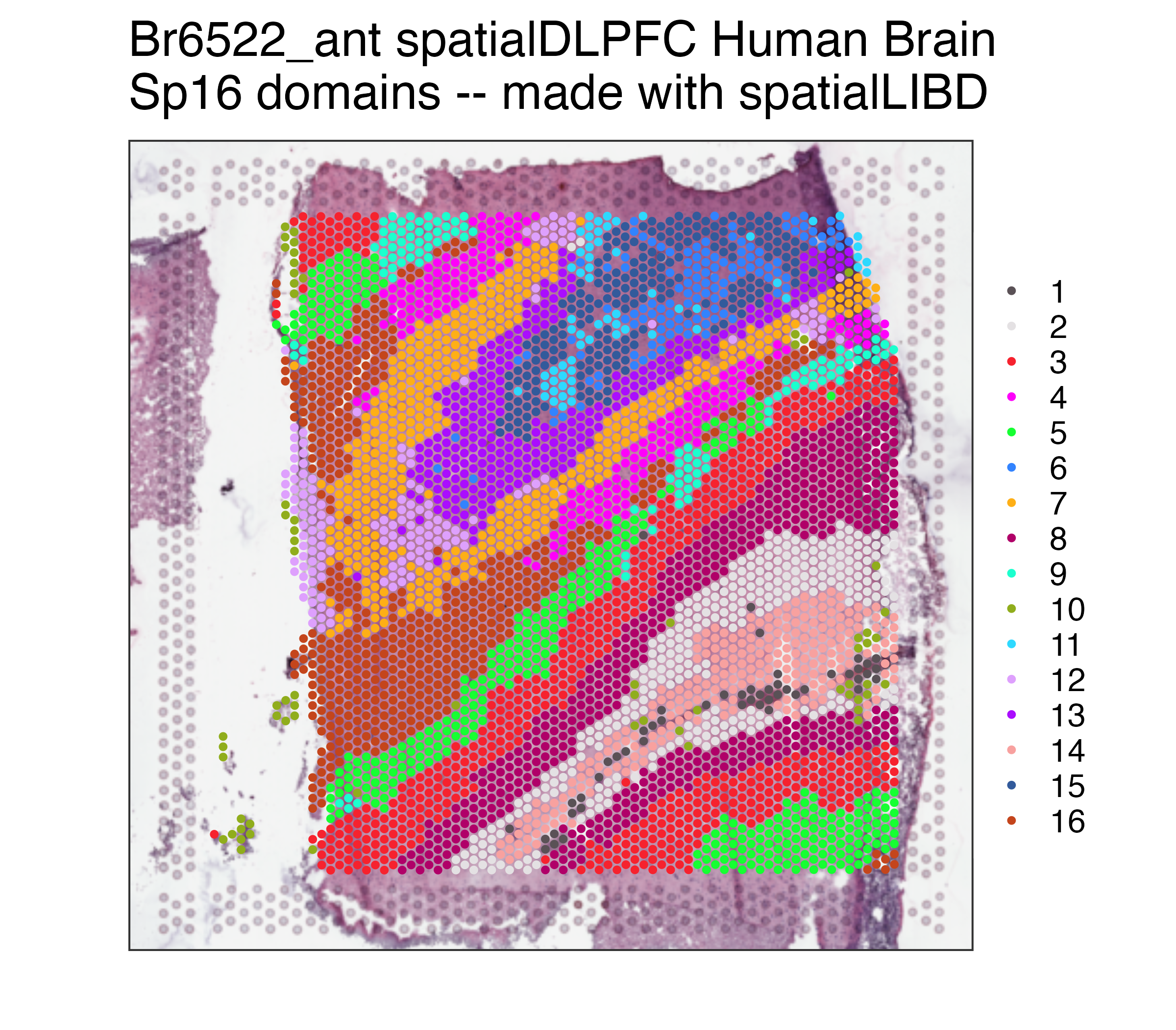
The source data described in this manuscript are available via the PsychENCODE Knowledge Portal (https://PsychENCODE.synapse.org/). The PsychENCODE Knowledge Portal is a platform for accessing data, analyses, and tools generated through grants funded by the National Institute of Mental Health (NIMH) PsychENCODE Consortium. Data is available for general research use according to the following requirements for data access and data attribution: (https://PsychENCODE.synapse.org/DataAccess). For access to content described in this manuscript see: https://doi.org/10.7303/syn51032055.1 or https://www.synapse.org/#!Synapse:syn51032055/datasets/. All figure and table files are available from https://www.synapse.org/#!Synapse:syn50908929.

You can also access all the raw data through Globus (jhpce#spatialDLPFC and jhpce#DLPFC_snRNAseq). This includes all the input FASTQ files as well as the outputs from tools such as SpaceRanger or CellRanger. The files are mostly organized following the LieberInstitute/template_project project structure.

Internal

  • JHPCE locations:
    • /dcs04/lieber/lcolladotor/spatialDLPFC_LIBD4035/spatialDLPFC
    • /dcs04/lieber/lcolladotor/deconvolution_LIBD4030/DLPFC_snRNAseq
  • Slack channel: libd_dlpfc_spatial.
  • code: R, python, and shell scripts for running various analyses.
    • spot_deconvo: cell-type deconvolution within Visium spots, enabled by tools like tangram, cell2location, cellpose, and SPOTlight
    • spython: older legacy testing scripts mostly replaced by spot_deconvo
  • plots: plots generated by RMarkdown or R analysis scripts in .pdf or .png format
  • processed-data
    • images_spatialLIBD: images used for running SpaceRanger
    • NextSeq: SpaceRanger output files
    • rdata: R objects
  • raw-data
    • FASTQ: FASTQ files from NextSeq runs.
    • FASTQ_renamed: renamed symbolic links to the original FASTQs, with consistent nomenclature
    • Images: raw images from the scanner in .tif format and around 3 GB per sample.
    • images_raw_align_json
    • psychENCODE: external data from PsychENCODE (doi: 10.7303/syn2787333).
    • sample_info: spreadsheet with information about samples (sample ID, sample name, slide serial number, capture area ID)

This GitHub repository is organized along the R/Bioconductor-powered Team Data Science group guidelines. It aims to follow the LieberInstitute/template_project structure, though most of the code/analysis output is saved at processed-data/rdata/spe directory unlike what’s specified in the template structure. This is due to historical reasons.

  • code: R scripts for running various analyses.
  • plots: plots generated by RMarkdown or R analysis scripts in .pdf or .png format
  • processed-data
    • cellranger: CellRanger output files
  • raw-data
    • FASTQ: FASTQ files.
    • sample_info: spreadsheet with information about samples (sample ID, sample name)

This GitHub repository is organized along the R/Bioconductor-powered Team Data Science group guidelines. It aims to follow the LieberInstitute/template_project structure.

Other related files

  • Reference transcriptome from 10x Genomics: /dcs04/lieber/lcolladotor/annotationFiles_LIBD001/10x/refdata-gex-GRCh38-2020-A/

spatialdlpfc's People

Stargazers

 avatar  avatar  avatar  avatar  avatar  avatar  avatar  avatar  avatar  avatar

Watchers

 avatar  avatar  avatar  avatar  avatar  avatar  avatar  avatar  avatar

spatialdlpfc's Issues

Compare new methods using our published data from 2021

Using the published data from 2021, compare the ARI from SpaGCN and BayesSpace (joint clustering). This will likely be a supplementary figure in this paper.

We should also add this info to our published data and its companion apps.

Move to trash any older rda files we don't need anymore

Move to trash/ any older SPE objects that we likely don't need anymore. The goal is to minimize confusion. You might want to do this before starting with #19.

That likely involves some of the spe objects listed at

$ ls -lh code/analysis/*rda
-rwxrwx--- 1 lcollado lieber_lcolladotor  28K Feb 10  2021 code/analysis/clusters_more_than_100_umis.rda
-rwxrwx--- 1 lcollado lieber_lcolladotor  30K Feb 10  2021 code/analysis/clusters_more_than_10_umis.rda
-rwxrwx--- 1 lcollado lieber_lcolladotor  30K Feb 10  2021 code/analysis/clusters_nonzero.rda
-rwxrwx--- 1 lcollado lieber_lcolladotor 162M Feb 15  2021 code/analysis/sce_combined.rda
-rwxrwx--- 1 lcollado lieber_lcolladotor 163M Jan 28  2021 code/analysis/sce_list.rda
-rwxrwx--- 1 lcollado lieber_lcolladotor 162M Feb 10  2021 code/analysis/sce_more_than_100_umis.rda
-rwxrwx--- 1 lcollado lieber_lcolladotor 162M Feb 10  2021 code/analysis/sce_more_than_10_umis.rda
-rwxrwx--- 1 lcollado lieber_lcolladotor 162M Feb 10  2021 code/analysis/sce_nonzero.rda

## Below we likely want to keep the metrics files, but not the spe or top.hvg ones
$ ls -lh processed-data/rdata/spe/*Rdata
-rw-rw---- 1 lcollado lieber_lcolladotor 1.7K Feb 17  2021 processed-data/rdata/spe/pilot_metrics.Rdata
-rw-rw---- 1 lcollado lieber_lcolladotor 2.7K Jul 27 11:06 processed-data/rdata/spe/sample_metrics_072721.Rdata
-rw-rw---- 1 lcollado lieber_lcolladotor 5.1K Jul 28 07:16 processed-data/rdata/spe/sample_metrics_all.Rdata
-rw-rw---- 1 lcollado lieber_lcolladotor 2.4K Feb 17  2021 processed-data/rdata/spe/sample_metrics.Rdata
-rw-rw---- 1 lcollado lieber_lcolladotor 4.5K Jul 27 12:15 processed-data/rdata/spe/shared_metrics_072721.Rdata
-rw-rw---- 1 lcollado lieber_lcolladotor 1.6K Feb 17  2021 processed-data/rdata/spe/shared_metrics.Rdata
-rw-rw---- 1 lcollado lieber_lcolladotor 840M Sep  1 12:34 processed-data/rdata/spe/spe_072821.Rdata
-rw-rw---- 1 lcollado lieber_lcolladotor 418M Jul 28 15:05 processed-data/rdata/spe/spe_raw_072821.Rdata
-rw-rw---- 1 lcollado lieber_lcolladotor 168M Feb 17  2021 processed-data/rdata/spe/spe_raw.Rdata
-rw-rw---- 1 lcollado lieber_lcolladotor 343M Feb 17  2021 processed-data/rdata/spe/spe.Rdata
-rw-rw---- 1 aspangle lieber_lcolladotor 138K Sep  1 11:17 processed-data/rdata/spe/top.hvgs_all.Rdata
-rw-rw---- 1 lcollado lieber_lcolladotor 114K Feb 17  2021 processed-data/rdata/spe/top.hvgs.Rdata

among other places.

Here's another way of finding these files based on https://stackoverflow.com/a/5905126/9374370:

## .rda files
$ find . -name "*.rda"
./code/analysis/clusters_more_than_10_umis.rda
./code/analysis/clusters_more_than_100_umis.rda
./code/analysis/sce_more_than_100_umis.rda
./code/analysis/sce_more_than_10_umis.rda
./code/analysis/clusters_nonzero.rda
./code/analysis/sce_combined.rda
./code/analysis/sce_nonzero.rda
./code/analysis/sce_list.rda

## .Rdata files
$ find . -name "*.Rdata"
./processed-data/rdata/inspect_scuttle_issue_7.Rdata
./processed-data/rdata/spe/spe.Rdata
./processed-data/rdata/spe/sample_metrics.Rdata
./processed-data/rdata/spe/spe_072821.Rdata
./processed-data/rdata/spe/spe_raw.Rdata
./processed-data/rdata/spe/shared_metrics_072721.Rdata
./processed-data/rdata/spe/top.hvgs.Rdata
./processed-data/rdata/spe/sample_metrics_all.Rdata
./processed-data/rdata/spe/sample_metrics_072721.Rdata
./processed-data/rdata/spe/shared_metrics.Rdata
./processed-data/rdata/spe/pilot_metrics.Rdata
./processed-data/rdata/spe/top.hvgs_all.Rdata
./processed-data/rdata/spe/spe_raw_072821.Rdata
./processed-data/rdata/g_k50.Rdata

run space ranger on round4 data

3 "new" samples
6432_ant_2
8325_mid_2
2720_ant_2

2 resequences
2720post
8667ant

1 missing resequence (emailed Linda)
6423mid

Re-organize files to match new project structure

Overall file structure ideas https://lcolladotor.github.io/bioc_team_ds/organizing-your-work.html

Live examples: https://github.com/LieberInstitute/Visium_IF_AD and the newer https://github.com/LieberInstitute/DLPFC_snRNAseq

See more on Slack at https://jhu-genomics.slack.com/archives/C01EA7VDJNT/p1630516674026100

Current status:

 $ ls -lh /dcs04/lieber/lcolladotor/spatialDLPFC_LIBD4035/spatialDLPFC
total 234K
drwxrws---  2 lcollado lieber_lcolladotor   31 Jul 28 10:47 analysis
drwxrws--- 14 lcollado lieber_lcolladotor   14 Nov 25  2020 FASTQ
drwxrws---  2 lcollado lieber_lcolladotor    2 Nov 18  2020 html
drwxrws---  8 lcollado lieber_lcolladotor    9 Jul 14 13:25 Images
drwxrws---  4 lcollado lieber_lcolladotor   16 Jul 23 16:53 images_raw_align_json
drwxrws---  4 lcollado lieber_lcolladotor    4 Feb 17  2021 outputs
drwxrws---  6 lcollado lieber_lcolladotor   35 Aug  3 09:08 plots
drwxrws---  3 lcollado lieber_lcolladotor    5 Mar 22 12:33 rdata
-rw-rw----  1 lcollado lieber_lcolladotor 1.8K Nov 18  2020 README.md
drwxrws---  2 lcollado lieber_lcolladotor    5 Jul 26 12:27 sample_info
drwxrws---  3 lcollado lieber_lcolladotor    3 Jul 26 11:01 scripts
-rw-rw----  1 lcollado lieber_lcolladotor  270 Feb 15  2021 spatialDLPFC.Rproj

More specifically:

scuttle quick cluster

Run internal scuttle code and extract the information that leads to the warning at https://github.com/LieberInstitute/spatialDLPFC/blob/main/analysis/01_build_SPE.R#L339-L356 so we can explore this information at https://github.com/LieberInstitute/spatialDLPFC/blob/main/analysis/01a_check_scran_quick_cluster.R as needed.

This is related to LTLA/scuttle#7 where we want to find out if we are using the correct statistics and if the workaround Aaron introduced in scuttle 1.1.15 is appropriate or not.

Update scaleFactors code

Read in the scale factors at

# spatial scale factors
file_scale <- file.path(dir_spatial, "scalefactors_json.json")
scalefactors <- fromJSON(file = file_scale)
before you read the tissue position info at
dir_spatial <- file.path(dir_outputs, sample_name, "outs", "spatial")
file_tisspos <- file.path(dir_spatial, "tissue_positions_list.csv")
df_tisspos <- read.csv(file_tisspos, header = FALSE,
col.names=c("barcode_id", "in_tissue", "array_row", "array_col",
"pxl_col_in_fullres", "pxl_row_in_fullres"))
since we need it for doing the multiplications at https://github.com/LieberInstitute/HumanPilot/blob/7e0f25188969913bc247b5d6c1c47c3ad94c6f15/Analysis/Layer_Notebook.R#L118-L119.

It would be similar to https://github.com/LieberInstitute/HumanPilot/blob/7e0f25188969913bc247b5d6c1c47c3ad94c6f15/Analysis/Layer_Notebook.R#L105

Add more gene information

Use the GTF file we used for aligning the data with SpaceRanger to add more information about the genes. Note that the genes might not be in the same order, but you can rely on the Ensembl Gene ID for ordering the data.

That is, the file at

# features
file_features <- file.path(dir_matrix, "features.tsv.gz")
df_features <- read.csv(file_features, sep = "\t", header = FALSE,
col.names = c("gene_id", "gene_name", "feature_type"))
is equivalent to the map object made at https://github.com/LieberInstitute/HumanPilot/blob/7e0f25188969913bc247b5d6c1c47c3ad94c6f15/Analysis/Layer_Notebook.R#L78-L80 (with different column names, but they could be made consistent). I don't know if the genes are in the same order across all images, but it would be worth double checking.

In any case, the rest of the gene info can be obtained from the annotation GTF file as in https://github.com/LieberInstitute/HumanPilot/blob/7e0f25188969913bc247b5d6c1c47c3ad94c6f15/Analysis/Layer_Notebook.R#L81-L87.

Try running the shiny app locally (on a laptop)

After #7, to try out the new sce object with spatialLIBD::run_app() we need to do a couple of things.

  1. Check the file size in RAM using pryr::object_size(sce) at JHPCE
  2. Transfer the data to your laptop: the sce object as well as the low resolution images
  3. Install R 4.0.3 with Bioconductor 3.12 (BiocManager::install(version = "3.12") + BiocManager::valid())
  4. Install spatialLIBD (BiocManager::install("spatialLIBD"))

Next, we can try to run the app using spatialLIBD::run_app() that has the following arguments https://github.com/LieberInstitute/spatialLIBD/blob/master/R/run_app.R#L49-L93.

We'll need to override several of them (aka, not use the defaults). In particular:

Then, the app should ideally (we'll see if there's code that needs to be changed) work on the "spot-level" tab. The "layer-level" tab will still show the older data.

perform spatially aware clustering method

use harmony dimension (instead of PCs) to run bayesspace, do on pilot dlpfc samples https://edward130603.github.io/BayesSpace/articles/joint_clustering.html. harmony seems to the best for batch correction.
try substitute to bayesspace which is called resept. https://www.biorxiv.org/content/10.1101/2021.07.08.451210v2
another alternative to bayesspace is SpaGCN https://www.biorxiv.org/content/10.1101/2020.11.30.405118v1, https://github.com/jianhuupenn/SpaGCN/blob/master/tutorial/tutorial_ez_mode.md#3-read-in-data, https://github.com/jianhuupenn/SpaGCN/blob/master/tutorial/tutorial.md

make down-sampled version of SPE object

spe$quadrant <- if(coord_x < 0 & coord_y > 0) "topleft" else if(....) spe$sample_quadrant <- paste0(spe$sampleid, "_", spe$quadrant) sample_quad_list <- rafalib::splitit(spe$sample_quadrant) selected_sample_quad <- unlist(lapply(sample_squad_list, sample, n = 250)) spe_subsampled <- spe[, selected_sample_quad]

Plot marker genes using spatialLIBD

Hi Abby,

Can you make the plots for the marker genes? That will involve updating https://github.com/LieberInstitute/spatialDLPFC/blob/32a14108b4ccc2210f1f8f63857d51f4847f6994/analysis/02_marker_genes.R as well as including the R session info as a comment at the bottom of the script.

It'll probably be good so you can practice using the new spatialLIBD version with functions such as vis_clus_gene(). Check also the git/GitHub history for that file to check how I tried to simplify the code. I haven't tested it myself, so there might be a typo here or something missing here or there.

Thanks!

Use older columns for the tissue position info

Instead of the column names at

col.names=c("barcode_id", "in_tissue", "array_row", "array_col",
"pxl_col_in_fullres", "pxl_row_in_fullres"))
(which are the ones used in the current release of SpatialExperiment) use the older names as in https://github.com/LieberInstitute/HumanPilot/blob/7e0f25188969913bc247b5d6c1c47c3ad94c6f15/Analysis/Layer_Notebook.R#L116 then do the same multiplications (using the scaled factors info from #1) https://github.com/LieberInstitute/HumanPilot/blob/7e0f25188969913bc247b5d6c1c47c3ad94c6f15/Analysis/Layer_Notebook.R#L118-L119.

Eventually, we want this info in the colData(sce) slot which Abby is doing at

col_data <- cbind(df_barcodes, df_tisspos_ord[, -1])
. Note that you still want to check the order as in
# note: check and/or re-order rows to make sure barcode IDs match in df_barcodes and df_tisspos
dim(df_barcodes)
dim(df_tisspos)
ord <- match(df_barcodes$barcode_id, df_tisspos$barcode_id)
df_tisspos_ord <- df_tisspos[ord, ]
dim(df_tisspos_ord)
stopifnot(nrow(df_barcodes) == nrow(df_tisspos_ord))
stopifnot(all(df_barcodes$barcode_id == df_tisspos_ord$barcode_id))
.

Run SpaGCN

Once #41 is done, we'll want to run SpaGCN on the 30 samples we'll use for this project.

Create a new SPE object without the 3 samples with poor histology

Once #40 is done continue here.

Likely start a new script for this.

  • Change the order of how you read the samples at
    sample_id = c(
    "DLPFC_Br2743_ant_manual_alignment",
    "DLPFC_Br2743_mid_manual_alignment_extra_reads",
    "DLPFC_Br2743_post_manual_alignment",
    "DLPFC_Br3942_ant_manual_alignment",
    "DLPFC_Br3942_mid_manual_alignment",
    "DLPFC_Br3942_post_manual_alignment",
    "DLPFC_Br6423_ant_manual_alignment_extra_reads",
    "DLPFC_Br6423_mid_manual_alignment",
    "DLPFC_Br6423_post_extra_reads",
    "DLPFC_Br8492_ant_manual_alignment",
    "DLPFC_Br8492_mid_manual_alignment_extra_reads",
    "DLPFC_Br8492_post_manual_alignment",
    "Round2/DLPFC_Br2720_ant_manual_alignment",
    "Round2/DLPFC_Br2720_mid_manual_alignment",
    "Round2/DLPFC_Br2720_post_extra_reads",
    "Round2/DLPFC_Br6432_ant_manual_alignment",
    "Round2/DLPFC_Br6432_mid_manual_alignment",
    "Round2/DLPFC_Br6432_post_manual_alignment",
    "Round3/DLPFC_Br6471_ant_manual_alignment_all",
    "Round3/DLPFC_Br6471_mid_manual_alignment_all",
    "Round3/DLPFC_Br6471_post_manual_alignment_all",
    "Round3/DLPFC_Br6522_ant_manual_alignment_all",
    "Round3/DLPFC_Br6522_mid_manual_alignment_all",
    "Round3/DLPFC_Br6522_post_manual_alignment_all",
    "Round3/DLPFC_Br8325_ant_manual_alignment_all",
    "Round3/DLPFC_Br8325_mid_manual_alignment_all",
    "Round3/DLPFC_Br8325_post_manual_alignment_all",
    "Round3/DLPFC_Br8667_ant_extra_reads",
    "Round3/DLPFC_Br8667_mid_manual_alignment_all",
    "Round3/DLPFC_Br8667_post_manual_alignment_all",
    "Round4/DLPFC_Br2720_ant_2",
    "Round4/DLPFC_Br6432_ant_2",
    "Round4/DLPFC_Br8325_mid_2"
    ),
    thinking about the grid of how you want to plot them later (Check in with @kmaynard12). To avoid code like https://github.com/LieberInstitute/Visium_IF_AD/blob/master/code/04_build_spe/initial_exploration.R#L13-L18 https://github.com/LieberInstitute/Visium_IF_AD/blob/master/code/04_build_spe/initial_exploration.R#L48-L67.
  • Use read10xVisiumWrapper() like at
    spe_wrapper <- read10xVisiumWrapper(
  • Read in the spot counts using code like from
    ## Read in cell counts and segmentation results
    segmentations_list <- lapply(sample_info$sample_id, function(sampleid) {
    current<-sample_info$sample_path[sample_info$sample_id==sampleid]
    file <- file.path(current, "spatial", "tissue_spot_counts.csv")
    if(!file.exists(file)) return(NULL)
    x <- read.csv(file)
    x$key <- paste0(x$barcode, "_", sampleid)
    return(x)
    })
    ## Merge them (once the these files are done, this could be replaced by an rbind)
    segmentations <- Reduce(function(...) merge(..., all = TRUE), segmentations_list[lengths(segmentations_list) > 0])
    ## Add the information
    segmentation_match <- match(spe_wrapper$key, segmentations$key)
    segmentation_info <- segmentations[segmentation_match, - which(colnames(segmentations) %in% c("barcode", "tissue", "row", "col", "imagerow", "imagecol", "key")), drop=FALSE]
    colData(spe_wrapper) <- cbind(colData(spe_wrapper), segmentation_info)
  • Run scran to have the QC info.
  • There's no need to remake the QC plots.
  • Compute PCs and UMAP.
  • Run just a single tSNE just to have it there.
  • Run HARMONY and BayesSpace.
  • Run graph-based clustering on the HARMONY dimensions.
  • Make a grid plot of the BayesSpace results.

Add reduced dimensions

Similar to #9, lets add to the sce object the reduced dimensions using the data from all the images in our sce object prior to #8 & #7. That involves running code Abby is familiar with already from https://github.com/LieberInstitute/HumanPilot/blob/master/Analysis/sce_scran.R#L80-L230.

Note that that code uses block = sce$subject_position which will be study-specific. If we have samples from the same donors, I would use block with something like block = subject. If we have spatial replicates, then we should use the original block = sce$subject_position (which you'll need to create first). This block argument is our way of telling scran our data structure (like the fact that our spots from a given set of images).

Add info useful for the shiny app

Re-run VistoSeg on the 2 problematic samples

Once SpaceRanger is done re-running for the 2 problematic samples, to be extra careful, we'll re-run VistoSeg to count the cells per spot in these 2 samples. They are:

  • sample 1:
    DLPFC_Br2743_ant_manual_alignment V19B23-075 A1 /dcs04/lieber/lcolladotor/spatialDLPFC_LIBD4035/spatialDLPFC/raw-data/Images/round1/Liebert_Institute_OTS-20-7690_rush_anterior_1.tif /dcs04/lieber/lcolladotor/spatialDLPFC_LIBD4035/spatialDLPFC/raw-data/images_raw_align_json/V19B23-075-A1_1_Br2743_ant_manual_alignment.json /dcs04/lieber/lcolladotor/spatialDLPFC_LIBD4035/spatialDLPFC/raw-data/FASTQ/2_DLPFC_Br3942_ant
  • sample 4
    DLPFC_Br3942_ant_manual_alignment V19B23-075 B1 /dcs04/lieber/lcolladotor/spatialDLPFC_LIBD4035/spatialDLPFC/raw-data/Images/round1/Liebert_Institute_OTS-20-7690_rush_anterior_2.tif /dcs04/lieber/lcolladotor/spatialDLPFC_LIBD4035/spatialDLPFC/raw-data/images_raw_align_json/V19B23-075-B1_2_Br3942_ant_manual_alignment.json /dcs04/lieber/lcolladotor/spatialDLPFC_LIBD4035/spatialDLPFC/raw-data/FASTQ/3_DLPFC_Br6423_ant

Sample 1 already finished running on SpaceRanger and you can find the output at /dcs04/lieber/lcolladotor/spatialDLPFC_LIBD4035/spatialDLPFC/processed-data/rerun_spaceranger/DLPFC_Br2743_ant_manual_alignment.

Sample 4 is queued at JHPCE. Once it's done, the output will be at /dcs04/lieber/lcolladotor/spatialDLPFC_LIBD4035/spatialDLPFC/processed-data/rerun_spaceranger/DLPFC_Br3942_ant_manual_alignment.

Thanks @heenadivecha!

Add variables to explore low quality spots from scran

Before #8 and likely also before #7, we'll want to add a few things to our sce object. One of them could be a (or more than one) discrete variable https://github.com/LieberInstitute/spatialLIBD/blob/master/R/run_app.R#L58 that tells us what were spots that scran's quality control checks (designed for scRNA-seq data, not Visium data) are of low quality and should be discarded. That is, running code like https://github.com/LieberInstitute/HumanPilot/blob/master/Analysis/sce_scran.R#L32-L33 then taking the outputs (which are logical vectors) and converting them to discrete variables (so factor or character).

Let's try this with the 3 columns in https://github.com/LieberInstitute/HumanPilot/blob/master/Analysis/sce_scran.R#L35. So something like:

sce$scran_discard <- factor(edit_me, levels = c("TRUE", "FALSE"))
sce$scran_low_lib_size <- ...
sce$low_n_features <- ...

This might be more relevant for the LC data than the DLPFC data. But it'll be good to check.

Combine sce_list into a single sce object

For that step, you'll likely need to use code from https://github.com/LieberInstitute/HumanPilot/blob/master/Analysis/convert_sce.R#L19-L20. Note that the tibbles for the images have to be combined which involves https://github.com/LieberInstitute/HumanPilot/blob/7e0f25188969913bc247b5d6c1c47c3ad94c6f15/Analysis/Layer_Notebook.R#L151 and https://github.com/LieberInstitute/HumanPilot/blob/master/Analysis/convert_sce.R#L20.

#5 could be done before or after the cbind() step.

You might have to manually create additional columns for the colData(sce) such as subject, position, replicate, subject_position although that is study-dependent. For example, sce$position gets created at https://github.com/LieberInstitute/HumanPilot/blob/master/Analysis/convert_sce.R#L58-L59.

Recommend Projects

  • React photo React

    A declarative, efficient, and flexible JavaScript library for building user interfaces.

  • Vue.js photo Vue.js

    🖖 Vue.js is a progressive, incrementally-adoptable JavaScript framework for building UI on the web.

  • Typescript photo Typescript

    TypeScript is a superset of JavaScript that compiles to clean JavaScript output.

  • TensorFlow photo TensorFlow

    An Open Source Machine Learning Framework for Everyone

  • Django photo Django

    The Web framework for perfectionists with deadlines.

  • D3 photo D3

    Bring data to life with SVG, Canvas and HTML. 📊📈🎉

Recommend Topics

  • javascript

    JavaScript (JS) is a lightweight interpreted programming language with first-class functions.

  • web

    Some thing interesting about web. New door for the world.

  • server

    A server is a program made to process requests and deliver data to clients.

  • Machine learning

    Machine learning is a way of modeling and interpreting data that allows a piece of software to respond intelligently.

  • Game

    Some thing interesting about game, make everyone happy.

Recommend Org

  • Facebook photo Facebook

    We are working to build community through open source technology. NB: members must have two-factor auth.

  • Microsoft photo Microsoft

    Open source projects and samples from Microsoft.

  • Google photo Google

    Google ❤️ Open Source for everyone.

  • D3 photo D3

    Data-Driven Documents codes.