jtsec92 / jt-blog Goto Github PK

View Code? Open in Web Editor NEW

0.0 1.0 0.0 1 KB

jt-blog's People

Contributors

Watchers

jt-blog's Issues

Exoplanet Classification using Machine Learning Techniques

slug: exoplanet-classification
date: 05-May-2024
summary: Classifed Kepler Objects of Interest (KOIs) from the NASA Exoplanet Archive dataset.
techStack: Python, Sci-Kit Learn, Pandas, Tensorflow
category: Personal Project
githubLink: https://github.com/klesser/cis600final
image: https://jt-portfolio-2024.s3.amazonaws.com/exoplanets.jpg

Introduction

The Kepler space telescope was launched on March 7th 2009, since then, data collected from the Kepler space telescope has been used to detect thousands of exoplanets and exoplanet candidates. Some of this data is maintained in the NASA Exoplanet Archive Planetary System dataset [Planetary Systems Dataset] which contains 26,329 rows planetary systems of which 4,154 are confirmed exoplanets - whereby the criteria for classifying the planet as an exoplanet by NASA is as follows [exoplanet criteria]:

The mass (or minimum mass) is equal to or less than 30 Jupiter masses.
The planet is not free floating.
Sufficient follow-up observations and validation have been undertaken to deem the possibility of the object being a false positive unlikely.
The above information along with further orbital and/or physical properties are available in peer-reviewed publications.

While more scientific approaches will always be necessary to confirm an exoplanet, the availability of this dataset combined with the importance of having tools that can separate the many objects in the observable universe from potentially habitable planets provides novice data scientists with sufficient reason to build a machine learning model that can aid astronomers and astrophysicists in their task of classifying exoplanets.

dataset = pd.read_csv('PS_2020.05.18_17.19.17.csv')

The 26,329 rows are loaded here and the 4,154 confirmed exoplanets are separated based on the binary 'default_flag' column. Therefore we can use the other columns in the dataset to train a machine learning model that can classify a planetary system as either an exoplanet or not an exoplanet. The exact CSV is available here.

Section 1: Data Preparation

null_matrix = msno.matrix(dataset)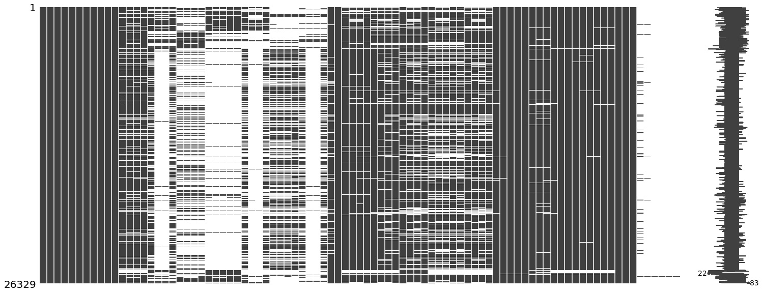

1.2 Cleaning

There were numerous types of values to be cleaned in the dataset. This included Msini, Mass where a numeric value should have been, HTML tags where there should not have been an HTML tag, and also some infinite values. These approaches led to positive accuracy rates however more granular approaches can be applied in the future.

# Cleaning - Remove String Values from Numeric Columns
dataset['pl_orbper'].replace(['</a>', '&'], np.nan, regex=True, inplace=True)
dataset['pl_orbpererr1'].replace(['</a>', '&'], np.nan, regex=True, inplace=True)
dataset['pl_orbpererr2'].replace(['</a>', '&'], np.nan, regex=True, inplace=True)
dataset['pl_orbeccen'].replace(['Msini', 'Mass'], np.nan, regex=True, inplace=True)
dataset['pl_orbeccenerr1'].replace(['Msini', 'Mass'], np.nan, regex=True, inplace=True)
dataset['pl_orbeccenerr2'].replace(['Msini', 'Mass'], np.nan, regex=True, inplace=True)
dataset['st_teff'].replace(['</a>', '&'], np.nan, regex=True, inplace=True)
dataset['st_tefferr1'].replace(['</a>', '&'], np.nan, regex=True, inplace=True)
dataset['st_tefferr2'].replace(['</a>', '&'], np.nan, regex=True, inplace=True)
dataset['st_tefflim'].replace(['</a>', '&'], np.nan, regex=True, inplace=True)
dataset['st_rad'].replace(['</a>', '&'], np.nan, regex=True, inplace=True)
dataset['st_raderr1'].replace(['</a>', '&'], np.nan, regex=True, inplace=True)
dataset['st_raderr2'].replace(['</a>', '&'], np.nan, regex=True, inplace=True)
dataset['st_logg'].replace(['[M/H]', '[Fe/H]'], np.nan, regex=True, inplace=True)
dataset['st_loggerr1'].replace(['[M/H]', '[Fe/H]'], np.nan, regex=True, inplace=True)
dataset['st_loggerr2'].replace(['[M/H]', '[Fe/H]'], np.nan, regex=True, inplace=True)
dataset['st_logglim'].replace(['[M/H]', '[Fe/H]'], np.nan, regex=True, inplace=True)
dataset['ra'].replace(['</a>', 's'], np.nan, regex=True, inplace=True)
dataset['dec'].replace(['</a>', 's'], np.nan, regex=True, inplace=True)
dataset['sy_dist'].replace(['</a>', 's'], np.nan, regex=True, inplace=True)
dataset['sy_disterr1'].replace(['</a>', 's'], np.nan, regex=True, inplace=True)
dataset['sy_disterr2'].replace(['</a>', 's'], np.nan, regex=True, inplace=True)
dataset['sy_vmag'].replace(['</a>', 's'], np.nan, regex=True, inplace=True)
dataset['sy_vmagerr1'].replace(['</a>', 's'], np.nan, regex=True, inplace=True)
dataset['sy_vmagerr2'].replace(['</a>', 's'], np.nan, regex=True, inplace=True)
dataset['default_flag'].replace([np.inf, -np.inf], np.nan)
dataset['default_flag'].dropna(inplace=True)

A number of columns were dropped including the right ascension of the planetary system in sexagesimal format as well as the declination of the planetary system in sexagesimal format due to conversion issues. Furthermore, ref_name columns and publication date columns were dropped due to the low probability that these columns were going to contribute to classification of KOIs into exoplanets - in addition conversion issues.

# All Columns Except for Target Column
X_train = dataset.iloc[:, 0:83].values
X_train = np.delete(X_train, 10, 1) # Drop pl_refname Column
X_train = np.delete(X_train, 40, 1) # Drop st_refname Column
X_train = np.delete(X_train, 61, 1) # Drop sy_refname Column
X_train = np.delete(X_train, 61, 1) # Drop rastr Column
X_train = np.delete(X_train, 62, 1) # Drop decstr Column
X_train = np.delete(X_train, 75, 1) # Drop rowupdate Column
X_train = np.delete(X_train, 75, 1) # Drop pl_pubdate Column
X_train = np.delete(X_train, 75, 1) # Drop releasedate Column

# Target Column (Exoplanet or not Exoplanet)
Y_train = dataset.iloc[:, 2:3].values

1.3 Impute Missing Values

Missing values were imputed in this section. The most frequent categorical value was added for categorical columns and the mean value was added for the numeric columns.

# Impute Missing Values for Purely Categorical Columns
imputer = SimpleImputer(missing_values=np.nan, strategy='most_frequent')
imputer = imputer.fit(X_train[:, [0,1,5,7,8,26,56]])
X_train[:, [0,1,5,7,8,26,56]] = imputer.transform(X_train[:, [0,1,5,7,8,26,56]])

# Impute Missing Values for Mixed/Numeric Type Columns
imputer = SimpleImputer(missing_values=np.nan, strategy='mean')
imputer = imputer.fit(X_train[:, [2,3,4,6,9,10,11,12,13]])
X_train[:, [2,3,4,6,9,10,11,12,13]] = imputer.transform(X_train[:, [2,3,4,6,9,10,11,12,13]])

imputer = imputer.fit(X_train[:, [14,15,16,17,18,19,20,21,22,23,24,25,27]])
X_train[:, [14,15,16,17,18,19,20,21,22,23,24,25,27]] = imputer.transform(X_train[:, [14,15,16,17,18,19,20,21,22,23,24,25,27]])

imputer = imputer.fit(X_train[:, [28,29,30,31,32,33,34,35,36,37,38]])
X_train[:, [28,29,30,31,32,33,34,35,36,37,38]] = imputer.transform(X_train[:, [28,29,30,31,32,33,34,35,36,37,38]])

imputer = imputer.fit(X_train[:, [39,40,41,42,43,44,45,46,47,48,49,50,51,52,53,54,55,55]])
X_train[:, [39,40,41,42,43,44,45,46,47,48,49,50,51,52,53,54,55,55]] = imputer.transform(X_train[:, [39,40,41,42,43,44,45,46,47,48,49,50,51,52,53,54,55,55]])

imputer = imputer.fit(X_train[:, [57,58,59,60,61,62,63,64,65,66,67,68,69,70,71]])
X_train[:, [57,58,59,60,61,62,63,64,65,66,67,68,69,70,71]] = imputer.transform(X_train[:, [57,58,59,60,61,62,63,64,65,66,67,68,69,70,71]])

imputer = imputer.fit(X_train[:, [72,73,74]])
X_train[:, [72,73,74]] = imputer.transform(X_train[:, [72,73,74]])

imputer_y = SimpleImputer(missing_values=np.nan, strategy='most_frequent')
imputer_y = imputer_y.fit(Y_train[:, [0]])
Y_train[:, [0]] = imputer_y.transform(Y_train[:, [0]])

1.4 Encode Categorical Values

# Convert Categorical Data to Numeric
labelencoder_X = LabelEncoder()
X_train[:, 0] = labelencoder_X.fit_transform(X_train[:, 0]) # pl_name - planet name
X_train[:, 1] = labelencoder_X.fit_transform(X_train[:, 1]) # hostname - hostname
X_train[:, 5] = labelencoder_X.fit_transform(X_train[:, 5]) # discoverymethod - discovery method
X_train[:, 7] = labelencoder_X.fit_transform(X_train[:, 7]) # discfacility - discovery facility
X_train[:, 8] = labelencoder_X.fit_transform(X_train[:, 8]) # soltype -
X_train[:, 26] = labelencoder_X.fit_transform(X_train[:, 26]) # pl_bmassprov -
X_train[:, 56] = labelencoder_X.fit_transform(X_train[:, 56]) # st_metratio -

1.5 Check NaN and Infinite Values

This is here to ensure that no NaN values or hanging infinity values are left in the data.

# Check if X_train contains any NaN values
array_X = np.array(X_train)
nan_check_X_train = np.any(pd.isnull(array_X))
print(nan_check_X_train)
print(np.isfinite(array_X.any()))

# Check if Y_train contains any NaN values
array_Y = np.array(Y_train)
nan_check_Y_train = np.any(pd.isnull(array_Y))
print(nan_check_Y_train)
print(np.isfinite(array_Y.any()))

1.6 Feature Selection

The data is split 75/25. 75% is used for training and 25% is used for testing. Furthermore, the 40 best predictors as chosen by the f_classif() and SelectKBest() functions. We found that passing non-feature scaled results to the neural network led to more positive results thus, feature scaled data is passed to most classifiers why non-feature scaled data was passed to the neural networks.

# Save X_train_nofs, X_test_nofs, X_test_nofs, and Y_test_nofs so all dimensions are passed to the neural network
X_train2 = X_train
Y_train2 = Y_train
X_train, X_test, Y_train, Y_test = train_test_split(X_train2, Y_train2.ravel(), test_size=0.25, random_state=0)
X_train_nofs = X_train
X_test_nofs = X_test
Y_train_nofs = Y_train
Y_test_nofs = Y_test

# Feature Selection for all other classifiers
X_new = SelectKBest(f_classif, k=40).fit_transform(X_train, Y_train.ravel())

1.7 Split Training Data

# Split features for all other classifiers
X_train, X_test, Y_train, Y_test = train_test_split(X_new, Y_train.ravel(), test_size=0.25, random_state=0)

1.8 Feature Scaling

# Feature Scaling
sc = StandardScaler()
X_train = sc.fit_transform(X_train)
X_test = sc.transform(X_test)

X_train_nn = sc.fit_transform(X_train_nn)
X_test_nn = sc.transform(X_test_nn)

1.9 Reduce Dimensionality using PCA

This code projects the 40 features onto a 5 dimensional subspace.

# Reduce Dimensionality using PCA
pca = PCA(n_components=5)
X_train = pca.fit_transform(X_train)
X_test = pca.transform(X_test)
explained_variance = pca.explained_variance_ratio_
print('Explained Variance: ', explained_variance)

Explained Variance: [0.18925958 0.10586026 0.08691283 0.05206524 0.0467069 ]

Section 2: Build, tune, and evaluate various machine learning algorithms

2.1 Create Gaussian Naive Bayes Classifier

#Create NB Classifiers
gnb_classifier = GaussianNB()
gnb_classifier.fit(X_train, Y_train.ravel())

GaussianNB(priors=None, var_smoothing=1e-09)

gnb_pred = gnb_classifier.predict(X_test)
gnb_cm = confusion_matrix(Y_test, gnb_pred)
gnb_accuracy = accuracy_score(Y_test, gnb_pred)
gnb_report = classification_report(Y_test, gnb_pred)
print(gnb_cm)
print(gnb_report)
print('GNB Accuracy: ', gnb_accuracy)

[[3754  406]
 [ 457  320]]
              precision    recall  f1-score   support

           0       0.89      0.90      0.90      4160
           1       0.44      0.41      0.43       777

    accuracy                           0.83      4937
   macro avg       0.67      0.66      0.66      4937
weighted avg       0.82      0.83      0.82      4937

GNB Accuracy:  0.8251974883532509

2.2 Create K-Nearest Neighbors Classifier

#Create K nearest neighbors classifier
knn_classifier = KNeighborsClassifier()
knn_classifier.fit(X_train,Y_train.ravel())

KNeighborsClassifier(algorithm='auto', leaf_size=30, metric='minkowski',
                     metric_params=None, n_jobs=None, n_neighbors=5, p=2,
                     weights='uniform')

knn_pred = knn_classifier.predict(X_test)
knn_cm = confusion_matrix(Y_test, knn_pred)
knn_accuracy = accuracy_score(Y_test, knn_pred)
print(knn_cm)
print('K-Nearest Accuracy: ', knn_accuracy)

[[4023  137]
 [ 180  597]]
K-Nearest Accuracy:  0.9357909661737898

Using GridSearchCV, we found that the best estimator used the Minkowski estimator with uniform weights and n_neighbors set to 5.

param_grid = {
    'n_neighbors' : [3,5,11,21,31,51],
    'weights' : ['uniform', 'distance'],
    'metric' : ['euclidean', 'manhattan']
}
knn_cv = GridSearchCV(KNeighborsClassifier(),param_grid,verbose=1,cv=3,n_jobs=-1)
knn_cv.fit(X_train, Y_train.ravel())

Fitting 3 folds for each of 24 candidates, totalling 72 fits
[Parallel(n_jobs=-1)]: Using backend LokyBackend with 8 concurrent workers.
[Parallel(n_jobs=-1)]: Done  34 tasks      | elapsed:    2.8s
[Parallel(n_jobs=-1)]: Done  72 out of  72 | elapsed:    4.4s finished

GridSearchCV(cv=3, error_score=nan,
             estimator=KNeighborsClassifier(algorithm='auto', leaf_size=30,
                                            metric='minkowski',
                                            metric_params=None, n_jobs=None,
                                            n_neighbors=5, p=2,
                                            weights='uniform'),
             iid='deprecated', n_jobs=-1,
             param_grid={'metric': ['euclidean', 'manhattan'],
                         'n_neighbors': [3, 5, 11, 21, 31, 51],
                         'weights': ['uniform', 'distance']},
             pre_dispatch='2*n_jobs', refit=True, return_train_score=False,
             scoring=None, verbose=1)

knn_cv_pred = knn_cv.predict(X_test)
knn_cv_cm = confusion_matrix(Y_test, knn_cv_pred)
knn_cv_accuracy = accuracy_score(Y_test, knn_cv_pred)
knn_cv_report = classification_report(Y_test, knn_cv_pred)
print(knn_cv_cm)
print(knn_cv_report)
print('Grid Search CV K-Nearest Accuracy: ', knn_cv_accuracy)
print('Grid Search CV K-Nearest Best Pararms: %s' % (knn_cv.best_params_))

[[4047 113]
[ 148 629]]
precision recall f1-score support

       0       0.96      0.97      0.97      4160
       1       0.85      0.81      0.83       777

accuracy                           0.95      4937

macro avg 0.91 0.89 0.90 4937
weighted avg 0.95 0.95 0.95 4937

Grid Search CV K-Nearest Accuracy: 0.9471338869758963
Grid Search CV K-Nearest Best Pararms: {'metric': 'manhattan', 'n_neighbors': 3, 'weights': 'distance'}

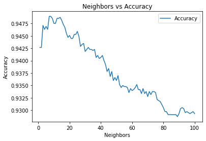
neighborsize = range(1,101)
results = []
for k in neighborsize:
    knn_n = KNeighborsClassifier(n_neighbors=k, weights='distance', metric='manhattan')
    knn_n.fit(X_train, Y_train.ravel())
    knn_pred_n = knn_n.predict(X_test)
    results.append(accuracy_score(Y_test, knn_pred_n))

points = list(zip(neighborsize,results))
knn_n_acc = pd.DataFrame(points, columns=['N','Accuracy']).set_index('N')
ax = sns.lineplot(data=knn_n_acc)
ax.set_title('Neighbors vs Accuracy')
ax.set_ylabel('Accuracy')
ax.set_xlabel('Neighbors')

Text(0.5, 0, 'Neighbors')

2.3 Create Random Forest Classifier

#Create Random Forest Classifier
rf_classifier = RandomForestClassifier()
rf_classifier.fit(X_train, Y_train.ravel())

RandomForestClassifier(bootstrap=True, ccp_alpha=0.0, class_weight=None,
                       criterion='gini', max_depth=None, max_features='auto',
                       max_leaf_nodes=None, max_samples=None,
                       min_impurity_decrease=0.0, min_impurity_split=None,
                       min_samples_leaf=1, min_samples_split=2,
                       min_weight_fraction_leaf=0.0, n_estimators=100,
                       n_jobs=None, oob_score=False, random_state=None,
                       verbose=0, warm_start=False)

rf_pred = rf_classifier.predict(X_test)
rf_cm = confusion_matrix(Y_test, rf_pred)
rf_accuracy = accuracy_score(Y_test, rf_pred)
rf_report = classification_report(Y_test, rf_pred)
print(rf_cm)
print('Random Forest Classifier Accuracy: ', rf_accuracy)
print('Random Forest Classifier Default Params: ', rf_classifier.get_params())

[[4077 83]
[ 137 640]]
Random Forest Classifier Accuracy: 0.9554385254202957
Random Forest Classifier Default Params: {'bootstrap': True, 'ccp_alpha': 0.0, 'class_weight': None, 'criterion': 'gini', 'max_depth': None, 'max_features': 'auto', 'max_leaf_nodes': None, 'max_samples': None, 'min_impurity_decrease': 0.0, 'min_impurity_split': None, 'min_samples_leaf': 1, 'min_samples_split': 2, 'min_weight_fraction_leaf': 0.0, 'n_estimators': 100, 'n_jobs': None, 'oob_score': False, 'random_state': None, 'verbose': 0, 'warm_start': False}

param_grid = {
    'n_estimators': [100, 500, 800],
    'max_features': ['auto', 'sqrt', 'log2'],
    'max_depth' : [5,10,None],
    'criterion' :['gini', 'entropy']
}
rfc_cv = GridSearchCV(estimator=RandomForestClassifier(), param_grid=param_grid, scoring='accuracy', cv=5, n_jobs=-1, verbose=1)
rfc_cv.fit(X_train,Y_train.ravel())

Fitting 5 folds for each of 54 candidates, totalling 270 fits
[Parallel(n_jobs=-1)]: Using backend LokyBackend with 8 concurrent workers.
[Parallel(n_jobs=-1)]: Done  34 tasks      | elapsed:   55.7s
[Parallel(n_jobs=-1)]: Done 184 tasks      | elapsed:  7.0min
[Parallel(n_jobs=-1)]: Done 270 out of 270 | elapsed: 12.6min finished

GridSearchCV(cv=5, error_score=nan,
             estimator=RandomForestClassifier(bootstrap=True, ccp_alpha=0.0,
                                              class_weight=None,
                                              criterion='gini', max_depth=None,
                                              max_features='auto',
                                              max_leaf_nodes=None,
                                              max_samples=None,
                                              min_impurity_decrease=0.0,
                                              min_impurity_split=None,
                                              min_samples_leaf=1,
                                              min_samples_split=2,
                                              min_weight_fraction_leaf=0.0,
                                              n_estimators=100, n_jobs=None,
                                              oob_score=False,
                                              random_state=None, verbose=0,
                                              warm_start=False),
             iid='deprecated', n_jobs=-1,
             param_grid={'criterion': ['gini', 'entropy'],
                         'max_depth': [5, 10, None],
                         'max_features': ['auto', 'sqrt', 'log2'],
                         'n_estimators': [100, 500, 800]},
             pre_dispatch='2*n_jobs', refit=True, return_train_score=False,
             scoring='accuracy', verbose=1)

rf_cv_pred = rfc_cv.predict(X_test)
rf_cv_cm = confusion_matrix(Y_test, rf_cv_pred)
rf_cv_accuracy = accuracy_score(Y_test, rf_cv_pred)
rf_cv_report = classification_report(Y_test, rf_pred)
print(rf_cv_cm)
print(rf_cv_report)
print('Random Forest Classifier Accuracy: ', rf_cv_accuracy)
print('Random Forest Classifier Best Params: ', rfc_cv.best_params_)

[[4076 84]
[ 123 654]]
precision recall f1-score support

       0       0.97      0.98      0.97      4160
       1       0.89      0.82      0.85       777

accuracy                           0.96      4937

macro avg 0.93 0.90 0.91 4937
weighted avg 0.95 0.96 0.95 4937

Random Forest Classifier Accuracy: 0.9580717034636419
Random Forest Classifier Best Params: {'criterion': 'entropy', 'max_depth': None, 'max_features': 'sqrt', 'n_estimators': 500}

df_x = pd.DataFrame.from_records(X_train)
tmp = pd.DataFrame({'Feature': df_x.columns, 'Feature importance': rf_classifier.feature_importances_})
tmp = tmp.sort_values(by='Feature importance',ascending=False)
plt.figure(figsize = (7,4))
plt.title('Random Forest Features Importance',fontsize=14)
s = sns.barplot(x='Feature',y='Feature importance',data=tmp)
s.set_xticklabels(s.get_xticklabels(),rotation=90)
plt.show()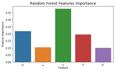

2.4 Create Gradient Boosting Machine Classifier

# Gradient Boosting Machine
gbm_classifier = GradientBoostingClassifier()
gbm_classifier.fit(X_train, Y_train.ravel())
y_pred_gbm = gbm_classifier.predict(X_test)
gbm_cm = confusion_matrix(Y_test, y_pred_gbm)
gbm_report = classification_report(Y_test, y_pred_gbm)
gbm_accuracy = accuracy_score(Y_test, y_pred_gbm)
print(gbm_report)
print('GBM Accuracy: ', gbm_accuracy)

              precision    recall  f1-score   support

           0       0.96      0.97      0.96      4160
           1       0.83      0.77      0.80       777

    accuracy                           0.94      4937
   macro avg       0.90      0.87      0.88      4937
weighted avg       0.94      0.94      0.94      4937

GBM Accuracy:  0.9392343528458578

param_grid = {
    # "loss":["deviance"],
    "learning_rate": [0.01, 0.025, 0.05, 0.075, 0.1, 0.15, 0.2],
    # "min_samples_split": np.linspace(0.1, 0.5, 12),
    # "min_samples_leaf": np.linspace(0.1, 0.5, 12),
    "max_depth":[3,5,8],
    "max_features":["log2","sqrt"],
    "subsample":[0.5, 0.618, 0.8, 0.85, 0.9, 0.95, 1.0],
    # "n_estimators":[10]
    }

gbm_cv = GridSearchCV(GradientBoostingClassifier(), param_grid=param_grid, cv=5, n_jobs=-1, verbose=1)
gbm_cv.fit(X_train, Y_train.ravel())
print(gbm_cv.best_params_)

Fitting 5 folds for each of 294 candidates, totalling 1470 fits

[Parallel(n_jobs=-1)]: Using backend LokyBackend with 8 concurrent workers.
[Parallel(n_jobs=-1)]: Done  34 tasks      | elapsed:   11.0s
[Parallel(n_jobs=-1)]: Done 184 tasks      | elapsed:  1.6min
[Parallel(n_jobs=-1)]: Done 434 tasks      | elapsed:  4.2min
[Parallel(n_jobs=-1)]: Done 784 tasks      | elapsed:  7.7min
[Parallel(n_jobs=-1)]: Done 1234 tasks      | elapsed: 12.4min
[Parallel(n_jobs=-1)]: Done 1470 out of 1470 | elapsed: 14.5min finished

{'learning_rate': 0.1, 'max_depth': 8, 'max_features': 'log2', 'subsample': 0.85}

gbm_cv_pred = gbm_cv.predict(X_test)
print(gbm_cv.best_params_)
print(f"Accuracy: {round(accuracy_score(Y_test, gbm_cv_pred)*100, 2)}%")
gbm_cv_report = classification_report(Y_test, gbm_cv_pred)
print(gbm_cv_report)
confusion_matrix(Y_test,gbm_cv_pred)

{'learning_rate': 0.1, 'max_depth': 8, 'max_features': 'log2', 'subsample': 0.85}\

Accuracy: 95.52%
              precision    recall  f1-score   support

           0       0.97      0.98      0.97      4160
           1       0.88      0.83      0.85       777

    accuracy                           0.96      4937
   macro avg       0.92      0.91      0.91      4937
weighted avg       0.95      0.96      0.95      4937

2.5 Create Artificial Neural Network Classifier

def create_ann():
    model = Sequential()
    model.add(Dense(units = 1, kernel_initializer = 'uniform', activation = 'sigmoid', input_dim = 75))
    model.compile(optimizer = 'adam', loss = 'binary_crossentropy', metrics = ['accuracy'])
    return model

ann0_classifier = KerasClassifier(build_fn=create_ann, epochs=50, batch_size=128, verbose=1, validation_split=0.25)
ann0_classifier._estimator_type = "classifier"
history_ann0 = ann0_classifier.fit(np.asarray(X_train_nofs).astype(np.float32), np.asarray(Y_train_nofs).astype(np.float32), batch_size = 128, epochs = 50, validation_split=0.25).history
y_pred_ann0 = ann0_classifier.predict(np.asarray(X_test_nofs).astype(np.float32), verbose=0)
y_pred_ann0 = (y_pred_ann0 > 0.5)
ann0_classifier.model.summary()

def create_ann1():
    model = Sequential()
    model.add(Dense(units = 6, kernel_initializer = 'uniform', activation = 'relu', input_dim = 75))
    model.add(Dense(units = 6, kernel_initializer = 'uniform', activation = 'relu'))
    model.add(Dense(units = 1, kernel_initializer = 'uniform', activation = 'sigmoid'))
    model.compile(optimizer = 'adam', loss = 'binary_crossentropy', metrics = ['accuracy'])
    return model

ann1_classifier = KerasClassifier(build_fn=create_ann1, epochs=50, batch_size=128, verbose=1, validation_split=0.25)
ann1_classifier._estimator_type = "classifier"
history_ann1 = ann1_classifier.fit(np.asarray(X_train_nofs).astype(np.float32), np.asarray(Y_train_nofs).astype(np.float32), batch_size = 128, epochs = 50, validation_split=0.25).history
y_pred_ann1 = ann1_classifier.predict(np.asarray(X_test_nofs).astype(np.float32), verbose=0)
y_pred_ann1 = (y_pred_ann1 > 0.5)
ann1_classifier.model.summary()

scores = ann0_classifier.model.evaluate(np.asarray(X_test_nofs).astype(np.float32), np.asarray(Y_test_nofs).astype(np.float32), verbose=0)
print("Accuracy: %.2f%%" % (scores[1]*100))

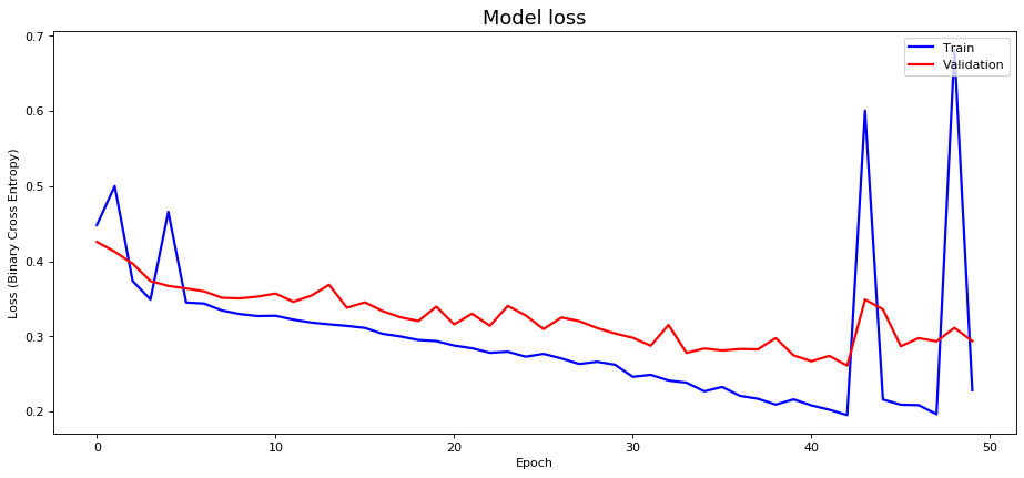
# plot training losses
fig10, ax10 = plt.subplots(figsize=(14, 6), dpi=80)
ax10.plot(history_ann1['loss'], 'b', label='Train', linewidth=2)
ax10.plot(history_ann1['val_loss'], 'r', label='Validation', linewidth=2)
ax10.set_title('Model loss', fontsize=16)
ax10.set_ylabel('Loss (Binary Cross Entropy)')
ax10.set_xlabel('Epoch')
ax10.legend(loc='upper right')
plt.show()

Accuracy: 91.34%

ann_report = classification_report(Y_test_nofs, y_pred_ann1)
print(ann_report)

              precision    recall  f1-score   support

           0       0.95      0.96      0.96      5552
           1       0.78      0.72      0.75      1031

    accuracy                           0.92      6583
   macro avg       0.86      0.84      0.85      6583
weighted avg       0.92      0.92      0.92      6583

Section 3: Metrics

3.1 Plot Receiver Operating Characteristic Curves

The KerasClassifier() wrapper function was added to the codebase to ensure that the artificial neural network classifiers were useable with the plot_roc_curve function although there is a slight bug with hanging ==== values.

gnb_disp = plot_roc_curve(gnb_classifier, X_test, Y_test, name='GNBClassifier')
ax1 = plt.gca()
knn_disp = plot_roc_curve(knn_cv, X_test, Y_test, ax=ax1, alpha=0.8, name='KNNClassifier')
ax2 = plt.gca()
rf_disp = plot_roc_curve(rfc_cv, X_test, Y_test, ax=ax2, alpha=0.8, name='RFClassifier')
ax3 = plt.gca()
gbm_disp = plot_roc_curve(gbm_classifier, X_test, Y_test, ax=ax3, alpha=0.8, name='GBMClassifier')
ax4 = plt.gca()
ann_disp = plot_roc_curve(ann0_classifier, np.asarray(X_train_nofs).astype(np.float32), np.asarray(Y_train_nofs).astype(np.float32), ax=ax4, alpha=0.8, name='ANNClassifier0Hidden')
ax5 = plt.gca()
ann1_disp = plot_roc_curve(ann1_classifier, np.asarray(X_train_nofs).astype(np.float32), np.asarray(Y_train_nofs).astype(np.float32), ax=ax5, alpha=0.8, name='ANNClassifier2Hidden')
ax6 = plt.gca()
plt.show()

Section 4: Conclusion

Overall, we found that Random Forest produced the best accuracy, however positive results were achieved using K-Nearest Neighbors, Gradient Boosting Machine, and Artificial Neural Networks as well. Furthermore, given the positive results of our findings, we believe that in the future, machine learning models can also be deployed on machines that collect raw (primary) astronomical data to solve classification or regression problems instead of being applied on the secondary datasets created by scientists.

Favorite Books

slug: favorite-books
summary: My favorite books.
date: 2024-May-05

Favorite Books

I've read some of these from beginning to end. Some of these were helpful and/or useful to me during tough moments. In no particular order:

The Art Spirit by Robert Henri -
Water, Rock & Time: The Geologic Story of Zion National Park -
Steve Jobs by Walter Isaacson -
Democracy in America - Reeve Translation - I don't think there is any book out there that describes the American social, political, and economic character as well as Democracy in America.
Advice To a Young Investigator by Santiago Ramon y Cajal -
On China by Henry Kissinger - Mr. Kissinger explained the differences between American Exceptionalism and Chinese Exceptionalism in the first few chapters - that is the difference between exceptionalism that is based on values and how Chinese exceptionalism is different. I didn't read the whole book.
Descent of Man by Charles Darwin -
On Writing by Stephen King -
The Cambridge Handbook of Expertise and Expert Performance by K. Anders Ericsson -

Want to Read

These were interesting to me because there are a lot of design patterns that repeat over and over again in software engineering. These were also interesting because of how they resonate with the idea that time is a flat circle.

Machine Learning Methods for Anomaly Detection in Industrial Control Systems

slug: anomaly-detection-ics
date: 05-May-2024
summary: Tested different anomaly detection models against the Kaggle HIL-based Augmented ICS (HAI) Security Dataset.
techStack: Python, Sci-Kit Learn, Pandas, Tensorflow
category: Personal Project
githubLink: https://github.com/jtsec92/CIS700_FinalMilestone
image: https://jt-portfolio-2024.s3.amazonaws.com/water-ics.jpg

Introduction

The following report explains various approaches that were evaluated for sequence classification of industrial control system data for the final project of CIS 700. In order to improve upon Milestone 2, these types of classifiers were evaluated or tuned:

Random Forest Classifier
Gradient Boosting Machine
Artificial Neural Network
LSTM
LSTM Autoencoder

And in order to attempt to reduce bias, a change was made in the preprocessing step to more closely follow the guidelines in A Survey of Data Mining and Machine Learning Methods for Cyber Security Intrusion Detection. The paper states that "in the case of anomaly detection, the normal traffic pattern is defined in the training phase. In the testing phase, the learned model is applied to new data, and every exemplar in the testing test is classified as either normal or anomalous". Therefore, instead of combining both normal and abnormal into one dataset and splitting which was the case for Milestone 2, the normal dataset is only used for training and the abnormal dataset is only used for testing.

Section 0 - Load Libraries, Load Data

Imports skipped.

dataset_abnorm1 = pd.read_csv('data/abnormal_20191029T110000_to_20191101T200000.csv')
dataset_abnorm2 = pd.read_csv('data/abnormal_20191104T150000_to_20191105T093000.csv')
dataset_norm1 = pd.read_csv('data/normal_20190911T200000_to_20190915T100000.csv')
dataset_norm2 = pd.read_csv('data/normal_20191101T200000_to_20191104T150000.csv')
dataset_norm1.dataframeName = 'normal_20191101T200000_to_20191104T150000.csv'

dataset_abnorm1['time'] = dataset_abnorm1['time'].astype(str).str[:-6].astype(np.str)
dataset_abnorm2['time'] = dataset_abnorm2['time'].astype(str).str[:-6].astype(np.str)
dataset_norm1["time"] = dataset_norm1['time'].astype(str).str[:-6].astype(np.str)
dataset_norm2["time"] = dataset_norm2['time'].astype(str).str[:-6].astype(np.str)

dataset_abnorm1['time'] = pd.to_datetime(dataset_abnorm1['time'])
dataset_abnorm2['time'] = pd.to_datetime(dataset_abnorm2['time'])
dataset_norm1["time"] = pd.to_datetime(dataset_norm1['time'])
dataset_norm2["time"] = pd.to_datetime(dataset_norm2['time'])

The following modification was made below in the preprocessing step to more clearly separate the normal data and abnormal data. In Milestone2 this section was combined into one whole dataset which may have increased bias. From the paper A Survey of Data Mining and Machine Learning Methods for Cyber Securtity Intrusion Detection: "in the case of anomaly detection, the normal traffic pattern is defined in the training phase. In the testing phase, the learned model is applied to new data, and every exemplar in the testing test is classified as either normal or anomalous".

# 09/11/2019 - 11/01/2019
# 11/01/2019 - 11/05/2019
combined = pd.concat([dataset_norm1, dataset_norm2])
combined_test = pd.concat([dataset_abnorm1, dataset_abnorm2])
combined.sort_values(by=['time'])

Far Left Columns

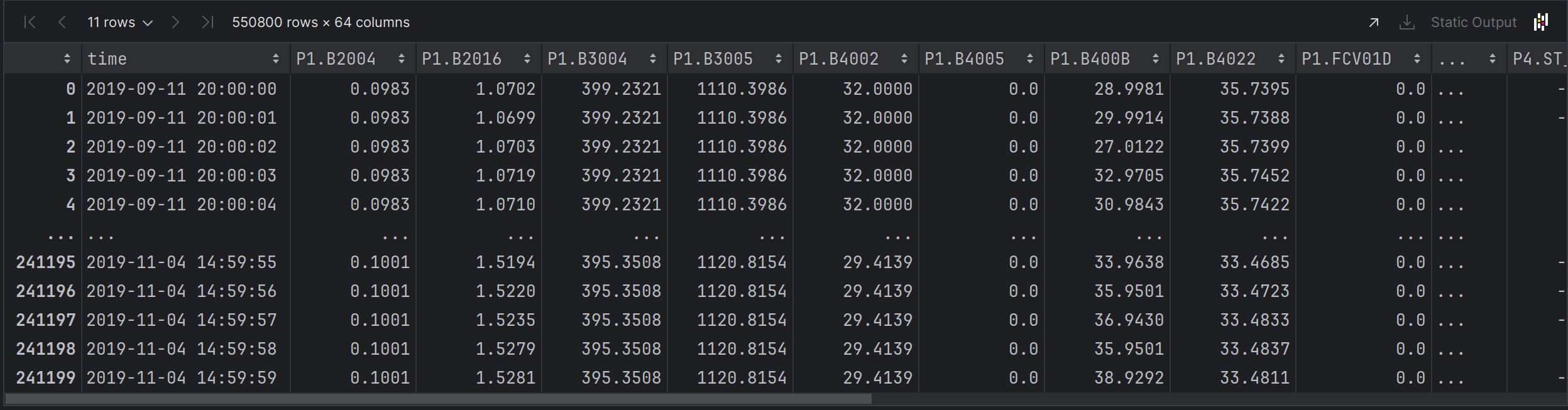
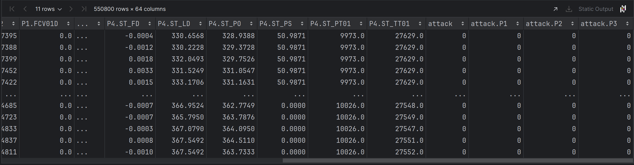
Far Right Columns

# X = P1, P2, P3, P4 Sensor Data
X = combined.iloc[:, 1:60].values
X_train = combined.iloc[:, 1:60].values
X_test = combined_test.iloc[:, 1:60].values

# Y = Attack Column
Y = combined.iloc[:, [61]].values
Y_train = combined.iloc[:, [61]].values
Y_test = combined_test.iloc[:, [61]].values

# Shape for LSTM
X_train_lstm = np.reshape(X_train, (X_train.shape[0], 1, X_train.shape[1]))
X_test_lstm = np.reshape(X_test, (X_test.shape[0], 1, X_test.shape[1]))

Section 1 - Feature Engineering

This code will select the 9 most relevant features from the training dataset and then grab the corresponding 9 features from the test dataset.

# Feature Selection
X_train_ensemble = SelectKBest(f_classif, k=9).fit_transform(X,Y)
X_new2 = SelectKBest(f_classif, k=9)
X_new2.fit(X_train, Y_train)

cols = X_new2.get_support(indices=True)
X_test_ensemble = combined_test.iloc[:,cols].values
features_df_new = combined_test.iloc[:,cols]
print(features_df_new)

       P2.SD01  P4.ST_PO  
0            0  349.6998  
1            0  349.8625  
2            0  350.4413  
3            0  350.6583  
4            0  352.4487  
...        ...       ...  
66595        0  333.3333  
66596        0  334.4546  
66597        0  334.8885  
66598        0  335.2503  
66599        0  335.8651  

[358200 rows x 9 columns]

sc = StandardScaler()
X_train_ensemble = sc.fit_transform(X_train_ensemble)
X_test_ensemble = sc.fit_transform(X_test_ensemble)

Section 2 - Model Creation

Gaussian Naive Bayes

# Gaussian Naive Bayes
gnb_classifier = GaussianNB()
gnb_classifier.fit(X_train, Y_train.ravel())
y_pred = gnb_classifier.predict(X_test)
gnb_cm = confusion_matrix(Y_test, y_pred)
gnb_accuracy = accuracy_score(Y_test, y_pred)
print('GNB Accuracy: ', gnb_accuracy)

GNB Accuracy:  0.5405248464544947

Random Forest

The number of trees in the forest is set to 20, the function for measuring impurity is set to Gini, the random state is set to 0, and n_jobs is set to -1 to use all CPU threads.

# Random Forest
rf_classifier0 = RandomForestClassifier(n_estimators = 20, criterion = 'gini', random_state = 0, verbose=1, n_jobs=-1)
rf_classifier0.fit(X_train_ensemble, Y_train.ravel())
y_pred_rf0 = rf_classifier0.predict(X_test_ensemble)
rf_cm = confusion_matrix(Y_test, y_pred_rf0)
rf_accuracy = accuracy_score(Y_test, y_pred_rf0)
print('RF Accuracy: ', rf_accuracy)

[Parallel(n_jobs=-1)]: Using backend ThreadingBackend with 16 concurrent workers.
[Parallel(n_jobs=-1)]: Done  10 out of  20 | elapsed:    0.6s remaining:    0.6s
[Parallel(n_jobs=-1)]: Done  20 out of  20 | elapsed:    0.9s finished
[Parallel(n_jobs=16)]: Using backend ThreadingBackend with 16 concurrent workers.
[Parallel(n_jobs=16)]: Done  10 out of  20 | elapsed:    0.1s remaining:    0.1s
[Parallel(n_jobs=16)]: Done  20 out of  20 | elapsed:    0.1s finished

RF Accuracy:  0.8293020658849805

GridSearchCV - Random Forest

# # GridSearchCV - Random Forest
rf_params = { 'n_estimators': [200, 500], 'max_features': ['auto', 'sqrt', 'log2'], 'max_depth' : [4,5,6,7,8], 'criterion' :['gini', 'entropy']}
rf_gscv_classifier_nofs = GridSearchCV(estimator=RandomForestClassifier(), param_grid=rf_params, verbose=1, cv=7, n_jobs=-1)
rf_gscv_classifier_nofs.fit(X_train_ensemble, Y_train.ravel())
y_pred_rf_gscv2 = rf_gscv_classifier.predict(X_train_ensemble)
rf_gscv_cm = confusion_matrix(Y_test, y_pred_rf_gscv2)
rf_gscv_accuracy = accuracy_score(Y_test, y_pred_rf_gscv2)
print('RF GSCV Accuracy Non Feature Scaled: ', rf_gscv_accuracy)
print('RF GSCV CM Non Featured Scaled: ', rf_gscv_cm)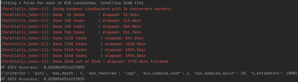

Random Forest Best Estimator

# Random Forest
rf_classifier8 = RandomForestClassifier(n_estimators = 1000, max_features='log2', min_samples_leaf=1, min_samples_split=10, criterion = 'gini', random_state=0, max_depth=4, verbose=1, n_jobs=-1)
rf_classifier8.fit(X_train_ensemble, Y_train.ravel())
y_pred_8 = rf_classifier8.predict(X_test_ensemble)
rf_cm = confusion_matrix(Y_test, y_pred_8)
rf_accuracy = accuracy_score(Y_test, y_pred_8)
print('RF Accuracy: ', rf_accuracy)

[Parallel(n_jobs=-1)]: Using backend ThreadingBackend with 16 concurrent workers.
[Parallel(n_jobs=-1)]: Done  18 tasks      | elapsed:    0.9s
[Parallel(n_jobs=-1)]: Done 168 tasks      | elapsed:    6.1s
[Parallel(n_jobs=-1)]: Done 418 tasks      | elapsed:   14.6s
[Parallel(n_jobs=-1)]: Done 768 tasks      | elapsed:   25.7s
[Parallel(n_jobs=-1)]: Done 1000 out of 1000 | elapsed:   33.3s finished
[Parallel(n_jobs=16)]: Using backend ThreadingBackend with 16 concurrent workers.
[Parallel(n_jobs=16)]: Done  18 tasks      | elapsed:    0.1s
[Parallel(n_jobs=16)]: Done 168 tasks      | elapsed:    0.6s
[Parallel(n_jobs=16)]: Done 418 tasks      | elapsed:    1.4s
[Parallel(n_jobs=16)]: Done 768 tasks      | elapsed:    2.6s
[Parallel(n_jobs=16)]: Done 1000 out of 1000 | elapsed:    3.4s finished

RF Accuracy:  0.8293467336683417

Gradient Boosting Machine

Uses all default values.

# Gradient Boosting Machine
gbm_classifier = GradientBoostingClassifier(verbose=1)
gbm_classifier.fit(X_train_ensemble, Y_train.ravel())
y_pred_gbm = gbm_classifier.predict(X_test_ensemble)
gbm_cm = confusion_matrix(Y_test, y_pred_gbm)
gbm_accuracy = accuracy_score(Y_test, y_pred_gbm)
print('GBM Accuracy: ', gbm_accuracy)
print('GBM CM: ,', gbm_cm)

      Iter       Train Loss   Remaining Time 
         1           0.0210           28.08s
         2           0.0204           39.34s
         3           0.0199           42.46s
         4           0.0197           43.70s
         5           0.0195           44.10s
         6           0.0193           44.36s
         7           0.0191           44.32s
         8           0.0187           46.81s
         9           0.0185           46.12s
        10           0.0184           45.66s
        20           0.0170           45.98s
        30           0.0164           41.94s
        40           0.0159           37.30s
        50           0.0155           32.21s
        60           0.0151           26.35s
        70           0.0148           19.98s
        80         265.9337           13.42s
        90         265.9320            6.69s
       100         266.3392            0.00s
GBM Accuracy:  0.7758598548297041
GBM CM: , [[265927  30618]
 [ 49669  11986]]

GridSearchCV - Gradient Boosting Machine

# GridSearchCV - Gradient Boosting Machine
gbm_parameters = {'max_depth':range(5,16,2), 'min_samples_split':range(200,1001,200)}
gbm_gscv_classifier = GridSearchCV(GradientBoostingClassifier(), gbm_parameters, verbose=1, cv=20, n_jobs=-1)
gbm_gscv_classifier.fit(X_train, Y_train.ravel())
y_pred = gbm_gscv_classifier.predict(X_test)
gbm_gscv_cm = confusion_matrix(Y_test, y_pred)
gbm_gscv_accuracy = accuracy_score(Y_test, y_pred)
print('GBM GSCV Accuracy: ', gbm_gscv_accuracy)
print(gbm_gscv_classifier.best_params_)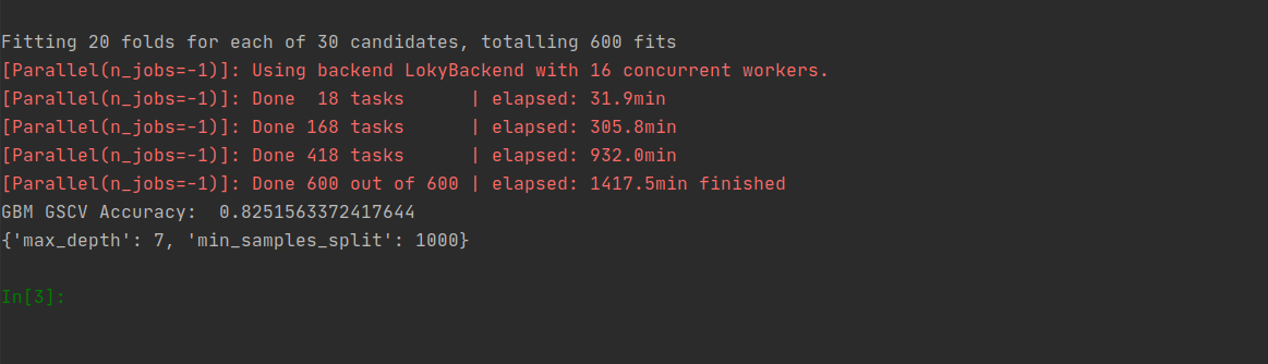

Gradient Boosting Machine Best Estimator

# Gradient Boosting Machine
gbm_classifier2 = GradientBoostingClassifier(max_depth=7, min_samples_split=1000, verbose=1)
gbm_classifier2.fit(X_train_ensemble, Y_train.ravel())
y_pred_gbm = gbm_classifier2.predict(X_test_ensemble)
gbm_cm = confusion_matrix(Y_test, y_pred_gbm)
gbm_accuracy = accuracy_score(Y_test, y_pred_gbm)
print('GBM Accuracy: ', gbm_accuracy)
print('GBM CM: ,', gbm_cm)

      Iter       Train Loss   Remaining Time 
         1           0.0216           29.03s
         2           0.0182            1.22m
         3           0.0129            1.45m
         4           0.0086            1.38m
         5           0.0082            1.32m
         6           0.0079            1.29m
         7           0.0075            1.26m
         8           0.0072            1.23m
         9           0.0069            1.21m
        10           0.0066            1.18m
        20           0.0050            1.32m
        30           0.0033            1.34m
        40 683565828765.1432           57.04s
        50 683565828765.1426           40.95s
        60 683565828765.1426           29.23s
        70 683565828765.1425           20.05s
        80 683565828765.1423           12.43s
        90 683565828765.1422            5.85s
       100 683565828765.1422            0.00s
GBM Accuracy:  0.8363149078726968
GBM CM: , [[296458     87]
 [ 58545   3110]]

Artificial Neural Network (3 Hidden Layers, 12 Nodes)

def create_ann():
    # create model
    model = Sequential()
    model.add(Dense(units = 12, kernel_initializer = 'uniform', activation = 'relu', input_dim = 59))
    model.add(Dense(units = 12, kernel_initializer = 'uniform', activation = 'relu'))
    model.add(Dense(units = 12, kernel_initializer = 'uniform', activation = 'relu'))
    model.add(Dense(units = 1, kernel_initializer = 'uniform', activation = 'sigmoid'))
    model.add(Dense(1, activation='sigmoid'))
    # Compile model
    model.compile(optimizer = 'adam', loss = 'binary_crossentropy', metrics = ['accuracy'])
    return model

ann3_classifier = KerasClassifier(build_fn=create_ann, epochs=5, batch_size=128, verbose=1, validation_split=0.25)
ann3_classifier._estimator_type = "classifier"
history_ann3 = ann3_classifier.fit(X_train, Y_train.ravel(), batch_size = 128, epochs = 5, validation_split=0.25).history
ann3_classifier.model.summary()

Training output omitted.

y_pred_ann3 = ann3_classifier.predict(np.asarray(X_test).astype(np.float32))
y_pred_ann3 = y_pred_ann3 > .5
y_pred_ann3 = y_pred_ann3 * 1
scores = ann3_classifier.model.evaluate(np.asarray(X_test).astype(np.float32), np.asarray(Y_test).astype(np.float32), verbose=0)
print("Accuracy: %.2f%%" % (scores[1]*100))

358200/358200 [==============================] - 2s 5us/sample
Accuracy: 82.79%

fig10, ax10 = plt.subplots(figsize=(14, 6), dpi=80)
ax10.plot(history_ann3['loss'], 'b', label='Train', linewidth=2)
ax10.plot(history_ann3['val_loss'], 'r', label='Validation', linewidth=2)
ax10.set_title('Model loss', fontsize=16)
ax10.set_ylabel('Loss (Binary Cross Entropy)')
ax10.set_xlabel('Epoch')
ax10.legend(loc='upper right')
plt.show()

Long Short-Term Memory (LSTM)

def simple_lstm():
    opt = SGD(lr=0.0001)
    model = Sequential()
    model.add(LSTM(10, input_shape=(1,59)))
    model.add(Dropout(0.2))
    model.add(Dense(1, activation='sigmoid'))
    model.compile(optimizer=opt, loss='binary_crossentropy', metrics=['accuracy'])
    return model

simple_lstm_model = KerasClassifier(build_fn=simple_lstm, epochs=5, batch_size=128, verbose=1, validation_split=0.25)
simple_lstm_model._estimator_type = "classifier"
history_simple_lstm = simple_lstm_model.fit(X_train_lstm, Y_train.ravel(), batch_size = 128, epochs = 5, validation_split=0.25, initial_epoch=1, use_multiprocessing=False).history
simple_lstm_model.model.summary()

Training output omitted.

scores = simple_lstm_model.model.evaluate(X_test_lstm, Y_test, verbose=1)
print("Accuracy: %.2f%%" % (scores[1]*100))

358200/358200 [==============================] - 19s 54us/sample - loss: 0.4592 - acc: 0.8279
Accuracy: 82.79%


```python
fig10, ax10 = plt.subplots(figsize=(14, 6), dpi=80)
ax10.plot(history_simple_lstm['loss'], 'b', label='Train', linewidth=2)
ax10.plot(history_simple_lstm['val_loss'], 'r', label='Validation', linewidth=2)
ax10.set_title('Model loss', fontsize=16)
ax10.set_ylabel('Loss (Binary Cross Entropy)')
ax10.set_xlabel('Epoch')
ax10.legend(loc='upper right')
plt.show()

Long Short-Term Memory (LSTM) Autoencoder

def autoencoder_model():
    opt = SGD(lr=0.0001)
    inputs = Input(shape=(1, 59))
    L1 = LSTM(16, activation='relu', return_sequences=True, kernel_regularizer=regularizers.l2(0.00))(inputs)
    L2 = LSTM(4, activation='relu', return_sequences=False)(L1)
    L3 = RepeatVector(1)(L2)
    L4 = LSTM(4, activation='relu', return_sequences=True)(L3)
    L5 = LSTM(16, activation='relu', return_sequences=True)(L4)
    L6 = LSTM(1, activation='sigmoid', return_sequences=True)(L5)
    output = TimeDistributed(Dense(59))(L6)
    model = Model(inputs=inputs, outputs=output)
    model.compile(optimizer=opt, loss='binary_crossentropy', metrics=['accuracy'])
    return model

lstm_autoencoder_model = KerasClassifier(build_fn=autoencoder_model, epochs=5, batch_size=128, verbose=1, validation_split=0.25)
lstm_autoencoder_model._estimator_type = "classifier"
history_autoencoder_lstm = lstm_autoencoder_model.fit(X_train_lstm, Y_train.ravel(), batch_size = 128, epochs = 5, validation_split=0.25, initial_epoch=1, use_multiprocessing=False).history
lstm_autoencoder_model.model.summary()

Training output omitted.

scores = lstm_autoencoder_model.model.evaluate(X_test_lstm, Y_test, verbose=1)
print("Accuracy: %.2f%%" % (scores[1]*100))

358200/358200 [==============================] - 48s 134us/sample - loss: 1.7553 - acc: 0.8279
Accuracy: 82.79%

fig10, ax10 = plt.subplots(figsize=(14, 6), dpi=80)
ax10.plot(history_autoencoder_lstm['loss'], 'b', label='Train', linewidth=2)
ax10.plot(history_autoencoder_lstm['val_loss'], 'r', label='Validation', linewidth=2)
ax10.set_title('Model loss', fontsize=16)
ax10.set_ylabel('Loss (Binary Cross Entropy)')
ax10.set_xlabel('Epoch')
ax10.legend(loc='upper right')
plt.show()

Section 3 - Performance Analysis

Thorough performance analysis: Results in data analysis can be misleading. Without detail analysis of different performance metrics (e.g. accuracy, recall, ROC, AUC, etc.) one-side view of results can present incomplete and inaccurate findings. Presenting a thorough analysis for overall performance of your models will show that you did not ignore any factor in your model.

Accuracy - Cross-Validated Mean

CV_Result = cross_val_score(rf_classifier0, X_test, Y_test, cv=5, n_jobs=-1, verbose=1)
print('RF0 - Cross-Validation Mean: ', CV_Result.mean())
print('RF0 - Cross-Validation Standard Deviation: ', CV_Result.std())

[Parallel(n_jobs=-1)]: Using backend LokyBackend with 16 concurrent workers.

RF0 - Cross-Validation Mean:  0.7640424343941932
RF0 - Cross-Validation Standard Deviation:  0.07406089942527304

[Parallel(n_jobs=-1)]: Done   5 out of   5 | elapsed:   20.4s finished

CV_Result = cross_val_score(rf_classifier8, X_test, Y_test, cv=5, n_jobs=-1, verbose=1)
print('RF0 - Cross-Validation Mean: ', CV_Result.mean())
print('RF0 - Cross-Validation Standard Deviation: ', CV_Result.std())

[Parallel(n_jobs=-1)]: Using backend LokyBackend with 16 concurrent workers.

RF0 - Cross-Validation Mean:  0.8651228364042435
RF0 - Cross-Validation Standard Deviation:  0.05436543216039365

[Parallel(n_jobs=-1)]: Done   5 out of   5 | elapsed:  3.7min finished

CV_Result = cross_val_score(gbm_classifier, X_test, Y_test, cv=5, n_jobs=-1, verbose=1)
print('GBM0 - Cross-Validation Mean: ', CV_Result.mean())
print('GBM0 - Cross-Validation Standard Deviation: ', CV_Result.std())

[Parallel(n_jobs=-1)]: Using backend LokyBackend with 16 concurrent workers.

GBM0 - Cross-Validation Mean:  0.836139028475712
GBM0 - Cross-Validation Standard Deviation:  0.07114835863111

[Parallel(n_jobs=-1)]: Done   5 out of   5 | elapsed:  6.0min finished

CV_Result = cross_val_score(gbm_classifier2, X_test, Y_test, cv=5, n_jobs=-1, verbose=1)
print('GBM0 - Cross-Validation Mean: ', CV_Result.mean())
print('GBM0 - Cross-Validation Standard Deviation: ', CV_Result.std())

[Parallel(n_jobs=-1)]: Using backend LokyBackend with 16 concurrent workers.
GBM0 - Cross-Validation Mean:  0.7722026800670017
GBM0 - Cross-Validation Standard Deviation:  0.10392960827997269
[Parallel(n_jobs=-1)]: Done   5 out of   5 | elapsed: 12.9min finished

CV_Result = cross_val_score(ann3_classifier, X_test, Y_test, cv=5, verbose=1)
print('ANN0 - Cross-Validation Mean: ', CV_Result.mean())
print('ANN0 - Cross-Validation Standard Deviation: ', CV_Result.std())

Training steps omitted.

ANN0 - Cross-Validation Mean:  0.857755446434021
ANN0 - Cross-Validation Standard Deviation:  0.05975990295410157
[Parallel(n_jobs=1)]: Done   5 out of   5 | elapsed:  2.6min finished

CV_Result = cross_val_score(simple_lstm_model, X_test_lstm, Y_test, cv=5, verbose=1)
print('ANN0 - Cross-Validation Mean: ', CV_Result.mean())
print('ANN0 - Cross-Validation Standard Deviation: ', CV_Result.std())

Training steps omitted.

ANN0 - Cross-Validation Mean:  0.8279564619064331
ANN0 - Cross-Validation Standard Deviation:  0.0001762128863227088
[Parallel(n_jobs=1)]: Done   5 out of   5 | elapsed:  4.6min finished

CV_Result = cross_val_score(lstm_autoencoder_model, X_test_lstm, Y_test, cv=5, verbose=1)
print('ANN0 - Cross-Validation Mean: ', CV_Result.mean())
print('ANN0 - Cross-Validation Standard Deviation: ', CV_Result.std())

Train on 214920 samples, validate on 71640 samples
...
ANN0 - Cross-Validation Mean:  0.8278861999511719
ANN0 - Cross-Validation Standard Deviation:  0.0001536130905151367
[Parallel(n_jobs=1)]: Done   5 out of   5 | elapsed: 13.6min finished

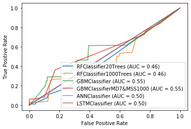
ROC Curve

disp = plot_roc_curve(rf_classifier0, X_test_ensemble, Y_test, name='RFClassifier20Trees')
ax1 = plt.gca()
rf_classifier8_disp = plot_roc_curve(rf_classifier8, X_test_ensemble, Y_test, ax=ax1, alpha=0.8, name='RFClassifier1000Trees')
ax2 = plt.gca()
gbm_classifier1_disp = plot_roc_curve(gbm_classifier, X_test_ensemble, Y_test, ax=ax2, alpha=0.8, name='GBMClassifier')
ax3 = plt.gca()
gbm_classifier2_disp = plot_roc_curve(gbm_classifier2, X_test_ensemble, Y_test, ax=ax3, alpha=0.8, name='GBMClassifierMD7&MSS1000')
ax4 = plt.gca()
ann_classifier1_disp = plot_roc_curve(ann3_classifier, X_test, Y_test, ax=ax4, alpha=0.8, name='ANNClassifier')
ax5 = plt.gca()
lstm_classifier1_disp = plot_roc_curve(simple_lstm_model, X_test_lstm, Y_test, ax=ax5, alpha=0.8, name='LSTMClassifier')
# ax6 = plt.gca()
# lstm_classifier2_disp = plot_roc_curve(lstm_autoencoder_model, X_test_lstm, Y_test, ax=ax6, alpha=0.8, name='LSTMAutoencoderClassifier')

[Parallel(n_jobs=16)]: Using backend ThreadingBackend with 16 concurrent workers.
[Parallel(n_jobs=16)]: Done  10 out of  20 | elapsed:    0.1s remaining:    0.1s
[Parallel(n_jobs=16)]: Done  20 out of  20 | elapsed:    0.1s finished
[Parallel(n_jobs=16)]: Using backend ThreadingBackend with 16 concurrent workers.
[Parallel(n_jobs=16)]: Done  18 tasks      | elapsed:    0.1s
[Parallel(n_jobs=16)]: Done 168 tasks      | elapsed:    0.7s
[Parallel(n_jobs=16)]: Done 418 tasks      | elapsed:    1.6s
[Parallel(n_jobs=16)]: Done 768 tasks      | elapsed:    2.9s
[Parallel(n_jobs=16)]: Done 1000 out of 1000 | elapsed:    3.7s finished

358200/358200 [==============================] - 3s 9us/sample
358200/358200 [==============================] - 5s 15us/sample

Accuracy

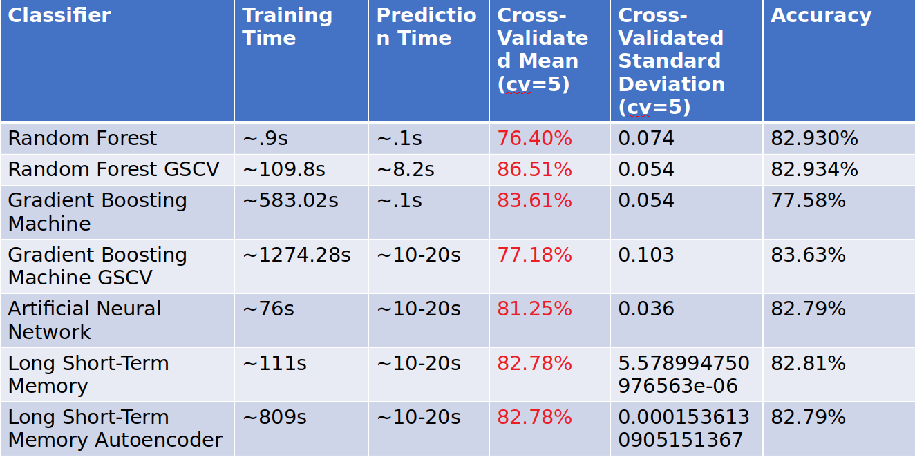
Model Execution Time

Model Execution Time (Partial, part of the final grading)
Many customers care about how long the winning models take to train and generate
predictions:

How long does it take to train your model? - Random Forest - .9s, Random Forest GSCV - 109.8s, Gradient Boosting Machine - 583.02s, Gradient Boosting Machine GSCV - ?, Artificial Neural Network - 76s, LSTM - 111s, LSTM Autoencoder 809s.
How long does it take to generate predictions using your model? - Random Forest - .1, Random Forest GSCV - 8.2s, Gradient Boosting Machine - .1s, Gradient Boosting Machine GSCV - 1274.28s, Artificial Neural Network - 10-20s, LSTM - 10-20s, LSTM Autoencoder 10-20s.
How long does it take to train the simplified model (referenced in section A6)? - Random Forest - .9s, Random Forest GSCV - 109.8s, Gradient Boosting Machine - 583.02s, Gradient Boosting Machine GSCV - 1274.28s, Artificial Neural Network - 76s, LSTM - 111s, LSTM Autoencoder 809s.
How long does it take to generate predictions from the simplified model? - Random Forest - .1, Random Forest GSCV - 8.2s, Gradient Boosting Machine - .1s, Gradient Boosting Machine GSCV - ?, Artificial Neural Network - 10-20s, LSTM - 10-20s, LSTM Autoencoder 10-20s.

Section 4 - Comparison Study

A Survey of Data Mining and Machine Learning Methods for Cyber Security Intrusion Detection. In the paper they survey different measures such as ANN, Associate Rules Bayesian Network, Clustering k-means, Clustering, hierarchical Clustering, DBSCAN Decision Trees, GA, Naive Bayes, K-Nearest Neighbors, HMM, Random Forest, and Support Vector Machines. The time complexities and ranges of accuracies gleaned from the document are shown in the table below:

Classifier	Typical Time Complexity	Accuracy
ANN	O(emnk)	Roughly 80% but varies
Association Rules	O(n³)	Roughly 100% with 13% FP Rate
Bayesian Network	O(mn)	93% with 1.39% FP Rate
Clustering, K-Means	O(kmni)	80%-90% but varies
Clustering, hierarchical	O(n³)	80%-90% but varies
Clustering, DBSCAN	O(n³)	80%-90% but varies
Decision Trees	O(mn²)	98.5% FAR was 0.9%
Genetic Algorithms (GA)	O(gkmn)	100% Best with FAR between 1.4% and 1.8%
Naive Bayes	O(mn)	Reported 98% and 89% accuracies
K-Nearest Neighbors	O(nlogk)	80%-90% but varies
Hidden Markov Models (HMM)	O(nc²)	Higher than 85%
Random Forest	O(Mmnlogn)	99% Range
Sequence Mining	O(n³)	Real-time scenario where 84% was detected
SVM	O(n²)	Results enhanced SVM "87.74%"

These are some of the ranges of accuracies using these approaches for binary classification of detect intrusions in various wired intrusion detection systems. These are in line with my results however some of these seem to be higher than 90% which is an improvement over my results. I would also assume that there are many false positives. I run a Fortinet Fortigate IDS system at home and I get many, many false positives. Furthermore, I cannot compare the Big-Oh notation times directly with my results because the output only shows as seconds or minutes.

Section 5 - Summary

Summarize the most important aspects of your model and analysis, such as:

The training method(s) you used (Convolutional Neural Network, XGBoost) - I used Random Forest, Gradient Boosting Machine, Artificial Neural Network, LSTM (Recurrent Neural Network), and LSTM Autoencoder (Recurrent Neural Network).
The most important features - The most important features were P1.B2004 (Boiler), P1.B3005 (Boiler), P1.FCV02Z (Boiler), P1.FCV03D (Boiler), P1.FCV03Z (Boiler), P1.PCV02D (Boiler), P2.On (Turbine), P2.SD01 (Turbine), P4.ST_P0 (HIL).
The tool(s) you used - I used Scikit-Learn, Keras, Matplotlib, Tensorflow, and other Python libraries. For the IDE I used Pycharm with Anaconda Plugin. For operating system I used Mac OSX and Ubuntu 18.04 LTS. To carry out testing I used Cross-Validated mean, ROC Curve, and accuracy metrics.
How long it takes to train your model - Random Forest - .9s, Random Forest GSCV - 109.8s, Gradient Boosting Machine - 583.02s, Gradient Boosting Machine GSCV - 583.02, Artificial Neural Network - 76s, LSTM - 111s, LSTM Autoencoder 809s.

Section 6 - Citations

Citations to references, websites, blog posts, and external sources of information
where appropriate.

Normally Keras does not integration well with scikit-learn. This tutorial shows how to combine KerasClassifiers and SciKit-Learn classifiers into models that can be passed to plot_roc_curve (https://machinelearningmastery.com/use-keras-deep-learning-models-scikit-learn-python/)
Long Short-Term Memory Networks by Jason Brownlee
Deep Learning Time Series Forecasting by Jason Brownlee
A Survey of Data Mining and Machine Learning Methods for Cyber Security Intrusion Detection

Section 7 - IEEE Paper

Link to the paper that was published in IEEE.

Appendix: Environment Setup

Version Control - Git
IDE - Pycharm with Anaconda Plugin
OS - Mac OSX
Packages - tensorflow (2.0.0), scikit-learn (0.22.1), etc.

Favorite Recipes 2024

slug: favorite-recipes-2024
summary: A few of my favorite recipes!
image: https://jt-portfolio-2024.s3.amazonaws.com/corncookies.webp
date: 2024-May-05

Baking

Cooking

Self-Study for Mathematics (2024-2028)

slug: math-self-study
summary: Plan for Self-Studying Mathematics
date: 2024-May-07

Plan by Year (Will Fix Table Formatting on the Website Later)

Topic	Book	Year (Est.)
Calculus I	Thomas Calculus: Early Transcendentals, 14th. Edition	2024 - 2025
Calculus II	Thomas Calculus: Early Transcendentals, 14th. Edition	2025 - 2026
Calculus III, Differential Equations	Thomas Calculus: Early Transcendentals; 14th. Edition A First Course in Differential Equations with Modeling Applications by Dennis Zill, 11th. Edition	2026 - 2028
Linear Algebra	Linear Algebra and Its Applications by David C. Lay, 6th Edition	2028?
Probability & Statistics	Introduction to Probability, Statistics, and Random Processes by Hossein Pishrok-Nik ; Introduction to Probability (Blitzstein & Hwang), 2nd Edition	?
Abstract Algebra	A First Course in Abstract Algebra by John B. Fraleigh	?
Real Analysis	Introduction to Real Analysis by Robert Bartle; Understanding Analysis by Abbott	?
Topology	?	?
Optimization	?	?

Nspect - Informed Purchasing Decisions through Supply Chain Insights

slug: nspect
date: 05-May-2024
summary: Nspect was envisioned as a tool that allowed consumers to see the country of origin for a product they were interested in purchasing.
techStack: Angular, Java
category: Personal Project
githubLink: https://github.com/jtsec92/webextension
image: https://jt-portfolio-2024.s3.amazonaws.com/supplychaininsights.webp

Summary

The code for this project is available at https://github.com/jtsec92/webextension.

The web extension was built for Chrome and was intended to scrape a product's SKU or ASIN from the Amazon HTML website and then perform a lookup of that product's country of origin in the event that the product's country of origin information was not already present on the page.

For example:

Zoomed Out

Zoomed In

However, due to how opaque the supply information for some products is as well as the sheer amount of hours that would need to be spent writing custom HTML for each product page type - this project was paused.

The Selenium Test in Action (GIF Below is Slow to Load)