TF2X is a self-educational project, exploring the computation graph and the the underlying computational model of Tensorflow. As the name suggests, the idea was to traverse the computation graph and convert it to other representations.
One rather straight forward idea was to convert to the computation
graph into executable code, e.g. JavaScript (in my defense I initiated
this project shortly before Tensorflow.JS was announced). TF2X offers
the tf2js method, that converts a Tensorflow graph to JavaScript code.
As of yet only a small subset of operations is supported but that subset
can be extended fairly easily.
TF2X contains a small example of an 99.3% MNIST classifier that is trained in Python and then converted to JS code, the result of which can be found here and the source code here.
The tf2js method takes a TF graph and converts it to a string containing
a JS class definition. Said class can be instantiated and then executed to
compute the individual graph nodes. The following example demonstates the
conversion from TF graph to JS and how to execute the result in NodeJS:
import numpy as np, os, subprocess, tensorflow as tf, tf2x
from pkg_resources import resource_string
from tempfile import mkdtemp
from tf2x import nd, tensor2js

ndjs_code = resource_string(tf2x.__name__, 'nd.js').decode('utf-8')

js_code_template = '''
{ND}
{Model}
const model = new MyModel()
const a_data = {a_data}
let output = model({{ 'a:0': a_data }})
console.log('\\nOutput JS:')
console.log( output.toString() )
'''

tf_a = tf.placeholder(name='a', shape=[3], dtype=tf.float32)
tf_b = tf.constant(10, name='b', dtype=tf.float32)
tf_c = tf_a + tf_b

with tf.Session() as sess:
  tf_out = sess.run( tf_c, feed_dict={ tf_a: [1,2,3] } )
  print('Output TF:')
  print( np.array2string( tf_out, separator=', ', max_line_width=256 ) )

  js_code = js_code_template.format(
    ND = ndjs_code,
    Model = tensor2js(tf_c, sess=sess, model_name='MyModel'),
    a_data = nd.arrayB64( np.array([1,2,3], dtype=np.float32) )
  )

js_dir = mkdtemp()
js_file = os.path.join(js_dir, 'main.js')

with open(js_file, 'w') as fout:
  fout.write(js_code)

proc = subprocess.Popen(['node', 'main.js'], stderr=subprocess.STDOUT, cwd=js_dir)
proc.wait()One of the main purposes of this project was to improve the understanding of Tensorflow's computational model. Good visualization of the graph is key to understanding. While the Tensorboard graph visualization gives an excellent overview over a large graph, it hides away quite a few details about the wiring of the graph on a low level. For those purposes, TF2X offers conversion method for the computation graph to both the Dot and GraphML format.
More ideas for the conversion of the TF graph were played around with but not (yet) implemented:
- TF Graph -> Spreadsheet
- TF Graph -> LaTex Math
In case the reader is interested in the TF computation graph, a few visualization examples are given in the following. The first example visualizes a simple graph with only a single binary operation:
import tensorflow as tf
from tf2x import tf2dot
from tempfile import mkdtemp

tf_a = tf.constant([1,2,3], dtype=tf.float32, name='a')
tf_b = tf.placeholder(      dtype=tf.float32, name='b')
tf_c = tf.add(tf_a,tf_b, name='c')

with tf.Session() as sess:
  dot = tf2dot( tf_c, sess=sess )

tmpdir = mkdtemp()
dot.format = 'png'
dot.render(directory=tmpdir, view=True)
Result:
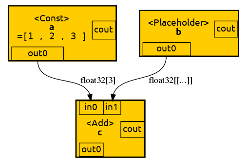
The computation graph for this simple example is pretty straight forward. We have a binary
operation c that has two input ports and a single output port. The output ports are what
is referred to as Tensor in TF graph mode. The first output of an operation a is addressed
as a:0 the second one as a:1, ... Furthermore it easy to believe that for
the operation c to be computed, operations a and b have to be computed first
as they are inputs of c. In other words c depends on a and b to be finished first.
(Note that in this example a and b are trivial to compute but in general they could be
complex subgraphs).
So far the computation graph is easy to grasp for everyone used to the Von-Neumann architecture (VNA). The second example shows how the Control-/Dataflow architecture used in TF graphs differs from VNA:
with tf.Graph().as_default() as graph:
  tf_a = tf.Variable([1,2,3], dtype=tf.float32, name='a')
  tf_b = tf.assign_add(tf_a, [4,5,6], name='b')

  init_vars = tf.global_variables_initializer()

  with tf.Session() as sess:
    dot = tf2dot( graph, sess=sess )

    sess.run(init_vars)

    result_a = sess.run(tf_a)
    print('A[0]:')
    print(result_a) # output: [1,2,3]

    sess.run(tf_b)
    sess.run(tf_b)

    result_a = sess.run(tf_a)
    print('A[1]:')
    print(result_a) # output: [9, 12, 15]

tmpdir = mkdtemp()

dot.format = 'png'
dot.attr( root='b:0' )
dot.render(directory=tmpdir, view=True)
Result:
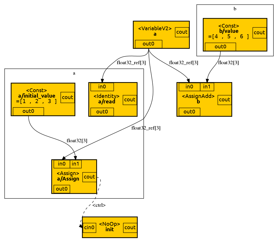
Let's ignore the initialization block on the lower left for now. It is interesting to note
that the VariableV2 operation block outputs a reference instead of a value. That makes
perfect sense if You consider that a variable is a mutable state stored somewhere in memory
that is subject to change.
For someone coming from VNA it may be unintuitve why result_a is [1,2,3] instead of
[5,7,9]. After all we have called assign_add in line 3, haven't we? Well, actually,
we haven't. In line 3, we merely created an operation that adds a value to a but we
haven't executed it yet. Only once we explicitly execute b using sess.run, we see
the variable state change. But what if we want the varible to be incremented before
every time we are reading it without having to call sess.run(tf_a) beforehand? Well,
that's were control dependencies come into play. In our first example the add operation
c was depending on a and b to be computed first. With control dependencies we
can artifically create such dependencies. The following example demonstrates that:
with tf.Graph().as_default() as graph:
  tf_a = tf.Variable([1,2,3], dtype=tf.float32, name='a')
  tf_b = tf.assign_add(tf_a, [4,5,6], name='b')
  with tf.control_dependencies([tf_b]):
    tf_c = tf.identity(tf_a, name='c')

  init_vars = tf.global_variables_initializer()

  with tf.Session() as sess:
    sess.run(init_vars)

    dot = tf2dot( graph, sess=sess )

    result_c = sess.run(tf_c)
    print('C[1]:', result_c) # output: [5. 7. 9.]

    result_c = sess.run(tf_c) # output: [ 9. 12. 15.]
    print('C[2]:', result_c)

tmpdir = mkdtemp()

dot.format = 'png'
dot.attr( root='b:0' )
dot.render(directory=tmpdir, view=True)
Result:
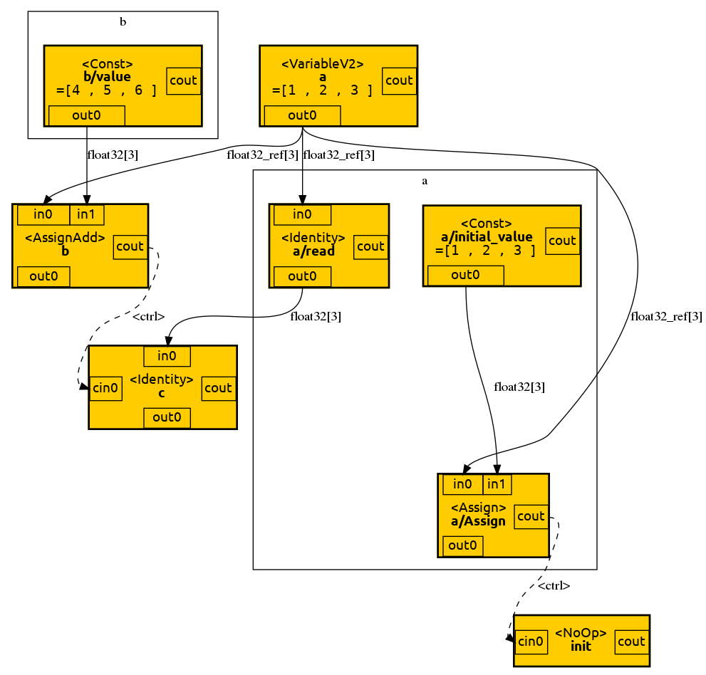
Note how the variable is incremented every time we read it. The identity operation c is used to wait until
b is finished before reading a. Note how the control depency is visible in the graph as a dashed line.
While in VNA the order of execution is deterministic and ordered, the only execution order in the Control-/Dataflow architecture is given by control and data dependencies. Other than that the graph may be executed in any order and
even in parallel (which makes this architecture so well suited for distributed computation). Let's now look
at how control structures are realized in a TF graph:
with tf.Graph().as_default() as graph:
  tf_a = tf.constant([1,2,3], dtype=tf.float32, name='a')
  tf_b = tf.constant([4,5,6], dtype=tf.float32, name='b')
  tf_c = tf.placeholder(shape=[], dtype=tf.bool, name='c')
  tf_d = tf.cond(tf_c, lambda: tf_a, lambda: tf_b, name='d')
  tf_e = tf.identity(tf_d, name='e')

  with tf.Session() as sess:
    dot = tf2dot( graph, sess=sess )

    result_e = sess.run(tf_d, feed_dict={tf_c: False})
    print('E(false):', result_e)

    result_e = sess.run(tf_d, feed_dict={tf_c: True })
    print('E(true):', result_e)

tmpdir = mkdtemp()

dot.format = 'png'
dot.attr( root='c:0' )
dot.render(directory=tmpdir, view=True)
Result:
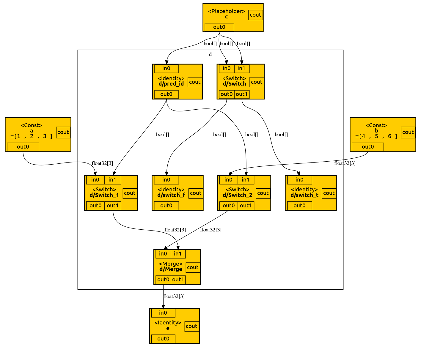
Sadly, the TF graph representation of a conditional is hard to identify a such. Let's ignore d/Switch,
d/Switch_t and d/Switch_f as they are unused in this case. The two new important operation types
in this graph are Switch and Merge. A Switch operation has two inputs and outputs. If the second
input (in1) value of a switch is false the first input value (in0) is forwarded to and emitted from
the first output port (out0). If the second input value of a switch is false the first input value
is forwarded to and emitted from the second output port (out1). The Merge operation takes inputs
from two ports (in0, in1) and forwards them to and emits them from a single output (out0).
Unfortunately, the TF graph representation of loops is even more involved:
tf_loop = tf.while_loop(
  cond = lambda i: i < tf.constant(16, name='iMax'),
  body = lambda i: i+1,
  loop_vars = (tf.constant(0, name='i0'),)
)
tf_out = tf.identity(tf_loop, name='out')

with tf.Session() as sess:
  dot = tf2dot( tf_out, sess=sess )

tmpdir = mkdtemp()

dot.format = 'png'
dot.attr( root='i0' )
dot.render(directory=tmpdir, view=True)
Result:
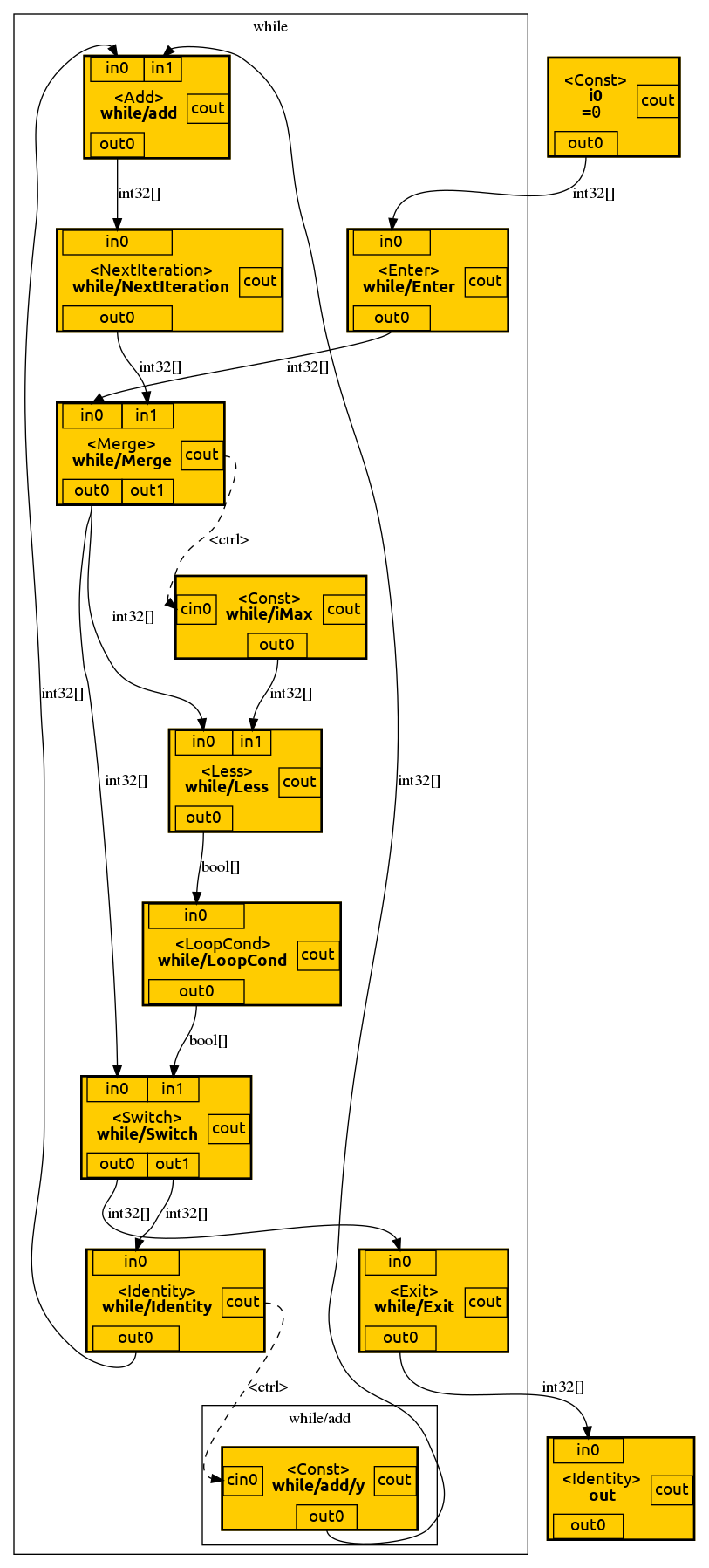
A loop statement is separated from the surrounding operations by Enter and Exit operations.
Next operations separate the individual loop iterations from one another. Note how - once again -
a Switch operations is used to conditionally used to decide wether to continue iteration or to
exit the loop. A more complete explaination of tf.while_loop, including its implementation,
can be found here.

