imchxx / blog Goto Github PK
View Code? Open in Web Editor NEW本repo主要是用作博客来记录日常学习、工作当中遇到的问题以及经验。
本repo主要是用作博客来记录日常学习、工作当中遇到的问题以及经验。


微信公众号开发者模式官方文档里以web.py作为例子,所以就打算按照教程来搭建自己的公众号。
本人系统为CentOS 6.10,Python版本为3.7。
[root@ichxx ~]# cat /etc/redhat-release
CentOS release 6.10 (Final)
(wx) [test@test wx]$ python -V
Python 3.7.0
按照web.py文档直接运行pip install web.py,结果报错了:
ModuleNotFoundError: No module named 'utils'ModuleNotFoundError: No module named 'db'分别安装utils和db模块后,安装的时候又报以下错误:
        print "var", var
                  ^
    SyntaxError: Missing parentheses in call to 'print'. Did you mean print("var", var)?
看到print "var", var,怀疑pip安装的是python 2的版本。搜了下在python 3里的安装方式。最后执行以下命令安装了web.py的dev版本成功。
pip install web.py==0.40.dev0
检查安装是否成功
(wx) [test@test dev]$ python
Python 3.7.0 (default, Sep 20 2018, 09:26:57)
[GCC 4.4.7 20120313 (Red Hat 4.4.7-18)] on linux
Type "help", "copyright", "credits" or "license" for more information.
>>> import web
>>>
win 10 家庭版安装numpy时报以下错误:
(data) D:\DATA\DEV\env\data>pip install numpy
Collecting numpy
  Downloading https://files.pythonhosted.org/packages/ed/29/d97b6252591da5f8add0d25eecda296ea72729a0aad7998edba1981b47c8/numpy-1.16.2-cp36-cp36m-win_amd64.whl (11.9MB)
    0% |                                | 10kB 467bytes/s eta 7:04:42Exception:
Traceback (most recent call last):
  File "d:\data\dev\env\data\lib\site-packages\pip\_vendor\urllib3\response.py", line 360, in _error_catcher
    yield
 ...
    raise ReadTimeoutError(self._pool, None, 'Read timed out.')
pip._vendor.urllib3.exceptions.ReadTimeoutError: HTTPSConnectionPool(host='files.pythonhosted.org', port=443): Read timed out.
从提示来看是由于超时了,安装时设置超时时间,问题解决。
(data) D:\DATA\DEV\env\data>pip install numpy --default-timeout=100
Collecting numpy
  Downloading https://files.pythonhosted.org/packages/ed/29/d97b6252591da5f8add0d25eecda296ea72729a0aad7998edba1981b47c8/numpy-1.16.2-cp36-cp36m-win_amd64.whl (11.9MB)
    100% |████████████████████████████████| 11.9MB 173kB/s
Installing collected packages: numpy
Successfully installed numpy-1.16.2
也可以使用国内的镜头源
pip install --index https://pypi.mirrors.ustc.edu.cn/simple/ pandas
注:--index后面也可以换成别的镜像,比如http://mirrors.sohu.com/python/
Pandas进行数据处理在前一章中,我们详细介绍了NumPy及其ndarray对象,它提供了Python中密集类型数组的高效存储和操作。在这里,我们将通过详细了解Pandas库提供的数据结构来构建这些知识。 Pandas是一个基于NumPy构建的新软件包,可以高效地实现DataFrame。DataFrames本质上是具有附加行和列标签的多维数组,并且通常具有异构类型和/或缺少数据。除了为标记数据提供方便的存储接口外,Pandas还实现了许多数据库框架和电子表格程序用户都熟悉的强大数据操作。
正如我们所看到的,NumPy的ndarray数据结构为数值计算任务中常见的统一,组织良好的数据类型提供了基本功能。虽然它很好地实现了这一目的,但当我们需要更多的灵活性时(例如,将标签附加到数据,处理缺失的数据等),它的局限性就变得清晰了,而且当尝试不能很好地映射到逐个元素的广播(例如,分组,枢轴等)的操作时,每次广播都是分析在我们周围的世界中以多种形式可用的结构较少的数据的重要部分。Pandas,特别是它的Series和DataFrame对象,建立在NumPy数组结构之上,可以高效访问这些占据数据科学家时间的“数据调整”任务。
在本章中,我们将重点介绍有效使用Series,DataFrame和相关结构的机制。我们将在适当的地方使用从真实数据集中提取的示例,但这些示例不一定是重点。
Pandas在系统上安装Pandas需要安装NumPy,如果从源代码构建库,则需要使用适当的工具来编译构建Pandas的C和Cython源。有关此安装的详细信息,请参阅Pandas文档。如果您遵循前言中概述的建议并使用Anaconda堆栈,则已安装Pandas。
安装Pandas后,您可以导入它并检查版本:
In [1]: import pandas
   ...: pandas.__version__
Out[1]: '0.24.1'
正如我们通常在别名np下导入NumPy一样,我们将在别名pd下导入Pandas:
In [2]: import pandas as pd
此导入约定将在本书的其余部分中使用。
在阅读本章时,不要忘记IPython使您能够快速浏览包的内容(通过使用制表符完成功能)以及各种功能的文档(使用?字符)。(如果您需要复习,请参阅IPython中的帮助和文档。)
例如,要显示pandas命名空间的所有内容,可以键入
In [3]: pd.<TAB>
要显示Pandas的内置文档,您可以使用:
In [4]: pd?
可以在http://pandas.pydata.org/上找到更详细的文档以及教程和其他资源。
使用Jupyter Notebook进行Matplotlib练习时,发现MatplotLib和Seaborn的版本比示例代码中的低

思考一会后,突然醒悟应该是由于练习使用的是虚拟环境,而Jupyter使用系统Python的原因吧。

网上搜了下,原生的Jupyter Notebook不支持使用虚拟环境。

如果想使用虚拟环境的话,需要安装一个插件conda install nb_conda

安装成功后,重启Jupyter Notebook,发现多了一个可选择的Python版本

然而,此Python [conda root] 环境根本不是我想使用的。我创建了多个虚拟玩意,这里都无法选择。

网上有人说,不是使用conda创建的虚拟环境还是选择不了。想起我的虚拟环境都是使用pip安装的virtualenv再创建的。
看了下另外的教程,先切换到虚拟环境,然后安装ipykernel,并将其加入到Jupyter内核中,重启后问题解决。
(data) e:\DEV\env\data\Scripts>pip install ipykernel
...
(data) e:\DEV\env\data\Scripts>python -m ipykernel install --user --name=data
Installed kernelspec data in C:\Users\test\AppData\Roaming\jupyter\kernels\data


conda安装的虚拟环境可以安装nb_conda,重启Jupyter即可解决。pip安装的先切换虚拟环境要安装ipykernel,然后再将其加入到Jupyter的内核,重启即可。网站上的计算机题目已经没有更新很久了,而且网站看起来比较简陋,应该没做什么反爬,所以就怎么简单怎么来,仅当练习。
# coding: utf-8
import time

import requests
from lxml import etree

# 入口
base_url = 'http://wap.ynpxrz.com/list.aspx?childid=2181&cateid=2160&page={}'
host = 'http://wap.ynpxrz.com'

def get_html(url):

    r = requests.get(url)
    if r.status_code == 200:
        return r
    return None

def get_parse(text):
    return etree.fromstring(text, parser=etree.HTMLParser())

def get_urls(page=1):
    url = base_url.format(page)
    r = get_html(url)
    if r:
        e = get_parse(r.text)
        url_tags = e.xpath('//*[@id="divList"]/li/a')
        urls = [host + url.get('href') for url in url_tags]
        return urls
    else:
        return None


def get_content(url):
    result = []
    r = requests.get(url)

    e = get_parse(r.text)
    # 标题
    h2_tags = e.xpath('/html/body/section/article/h2')
    title = h2_tags[0].text

    result.append(title)
    # 获取不含属性的节点
    p_tags = e.xpath('/html/body/section/article/div/p[not(@*)]')

    for tag in p_tags:
        if tag.text:
            result.append(tag.text.replace('更多信息请查看', ''))
    return result


if __name__ == '__main__':

    result = []
    page = 1
    print('开始')
    while page <= 23:
        urls = get_urls(page)
        for url in urls:
            content = get_content(url)
            title = content[0]
            print('page{}-{}'.format(page, title))
            result.append('\n'.join(content))
            result.append('--'*20)
            result.append('\n\n')
            time.sleep(1)
        # 生成文件
        with open('./data/page{}.txt'.format(page), 'w', encoding='utf-8') as f:
            f.write('\n'.join(result))
        # 重置result
        result = []
        page += 1
    print('结束')
cat /etc/issue
# redhat专用
cat /etc/redhat-release
uname -a
Python中的数据操作几乎与NumPy数组操作同义:即使是像Pandas(第3章)这样的新工具也是围绕NumPy数组构建的。本节将介绍使用NumPy数组操作访问数据和子数组,以及拆分,重新整形和连接数组的几个示例。虽然这里显示的操作类型可能看起来有点干燥和迂腐,但它们构成了本书中使用的许多其他示例的构建块。快点了解它们!
我们将在这里介绍几类基本数组操作:
NumPy数组属性首先让我们讨论一些有用的数组属性。我们首先定义三个随机数组,一维,二维和三维数组。我们将使用NumPy的随机数生成器,我们将使用设定值播种,以确保每次运行此代码时生成相同的随机数组:
In [1]: import numpy as np
   ...: np.random.seed(0)  # seed for reproducibility
   ...:
   ...: x1 = np.random.randint(10, size=6)  # One-dimensional array
   ...: x2 = np.random.randint(10, size=(3, 4))  # Two-dimensional array
   ...: x3 = np.random.randint(10, size=(3, 4, 5))  # Three-dimensional array
每个数组都有属性ndim(维度数),shape(每个维度的大小)和size(数组的总大小):
In [2]: print("x3 ndim: ", x3.ndim)
   ...: print("x3 shape:", x3.shape)
   ...: print("x3 size: ", x3.size)
x3 ndim:  3
x3 shape: (3, 4, 5)
x3 size:  60
另一个有用的属性是dtype,即数组的数据类型(我们之前在Python中理解数据类型中讨论过):
In [3]: print("dtype:", x3.dtype)
dtype: int32
其他属性包括itemsize,列出每个数组元素的大小(以字节为单位),nbytes列出数组的总大小(以字节为单位):
In [4]: print("itemsize:", x3.itemsize, "bytes")
   ...: print("nbytes:", x3.nbytes, "bytes")
itemsize: 4 bytes
nbytes: 240 bytes
通常,我们期望nbytes等于itemsize * size。
如果您熟悉Python的标准列表索引,NumPy中的索引将会非常熟悉。在一维数组中,可以通过在方括号中指定所需的索引来访问第i个值(从0开始计数),就像使用Python列表一样:
In [5]: x1
Out[5]: array([5, 0, 3, 3, 7, 9])

In [6]: x1[0]
Out[6]: 5

In [7]: x1[4]
Out[7]: 7
要从数组的末尾开始索引,可以使用负索引:
In [8]: x1[-1]
Out[8]: 9

In [9]: x1[-2]
Out[9]: 7
在多维数组中,可以使用以逗号分隔的索引元组来访问项:
In [10]: x2
Out[10]:
array([[3, 5, 2, 4],
       [7, 6, 8, 8],
       [1, 6, 7, 7]])

In [11]: x2[0, 0]
Out[11]: 3

In [12]: x2[2, 0]
Out[12]: 1

In [13]: x2[2, -1]
Out[13]: 7
也可以使用以上任何索引表示法修改值:
In [14]: x2[0, 0] = 12
    ...: x2
Out[14]:
array([[12,  5,  2,  4],
       [ 7,  6,  8,  8],
       [ 1,  6,  7,  7]])
请记住,与Python列表不同,NumPy数组具有固定类型。这意味着,例如,如果您尝试将浮点值插入整数数组,则将以静默方式截断该值。不要忽视这种行为!
In [15]: x1[0] = 3.14159  # this will be truncated!
    ...: x1
Out[15]: array([3, 0, 3, 3, 7, 9])
就像我们可以使用方括号来访问单个数组元素一样,我们也可以使用它们来访问带有切片表示法的子数组,并用冒号(:)字符标记。NumPy切片语法遵循标准Python列表的语法;要访问数组x的切片,请使用:
x[start:stop:step]
如果未指定其中任何一个,则默认为值start = 0,stop = 数组大小,step = 1。我们将看一下在一维和多维中访问子数组。
In [16]: x = np.arange(10)
    ...: x
Out[16]: array([0, 1, 2, 3, 4, 5, 6, 7, 8, 9])

In [17]: x[:5]  # first five elements
Out[17]: array([0, 1, 2, 3, 4])

In [18]: x[5:]  # elements after index 5
Out[18]: array([5, 6, 7, 8, 9])

In [19]: x[4:7]  # middle sub-array
Out[19]: array([4, 5, 6])

In [20]: x[::2]  # every other element
Out[20]: array([0, 2, 4, 6, 8])

In [21]: x[1::2]  # every other element, starting at index 1
Out[21]: array([1, 3, 5, 7, 9])
一个可能令人困惑的情况是步长值为负值。在这种情况下,开始和结束的默认值会交换。这成为反转数组的一种便捷方法:
In [22]: x[::-1]  # all elements, reversed
Out[22]: array([9, 8, 7, 6, 5, 4, 3, 2, 1, 0])

In [23]: x[5::-2]  # reversed every other from index 5
Out[23]: array([5, 3, 1])
In [24]: x2
Out[24]:
array([[12,  5,  2,  4],
       [ 7,  6,  8,  8],
       [ 1,  6,  7,  7]])

In [25]: x2[:2, :3]  # two rows, three columns
Out[25]:
array([[12,  5,  2],
       [ 7,  6,  8]])

In [26]: x2[:3, ::2]  # all rows, every other column
Out[26]:
array([[12,  2],
       [ 7,  8],
       [ 1,  7]])
最后,子数组的维度甚至可以一起反转:
In [27]: x2[::-1, ::-1]
Out[27]:
array([[ 7,  7,  6,  1],
       [ 8,  8,  6,  7],
       [ 4,  2,  5, 12]])
一个常用的例程是访问数组的单个行或列。这可以通过组合索引和切片来完成,使用由单个冒号(:)标记的空切片:
In [28]: print(x2[:, 0])  # first column of x2
[12  7  1]

In [29]: print(x2[0, :])  # first row of x2
[12  5  2  4]
在行访问的情况下,可以省略空切片以获得更紧凑的语法:
In [30]: print(x2[0])  # equivalent to x2[0, :]
[12  5  2  4]
了解数组切片的一个重要且非常有用的事情是它们返回视图而不是数组数据的副本。这是NumPy数组切片与Python列表切片不同的一个区域:在列表中,切片将是副本。考虑我们之前的二维数组:
In [31]: print(x2)
[[12  5  2  4]
 [ 7  6  8  8]
 [ 1  6  7  7]]
让我们从中提取一个2×2子数组:
In [32]: x2_sub = x2[:2, :2]
    ...: print(x2_sub)
[[12  5]
 [ 7  6]]
现在,如果我们修改这个子数组,我们会看到原始数组已经改变了!注意:
In [33]: x2_sub[0, 0] = 99
    ...: print(x2_sub)
[[99  5]
 [ 7  6]]

In [34]: print(x2)
[[99  5  2  4]
 [ 7  6  8  8]
 [ 1  6  7  7]]
这种默认行为实际上非常有用:这意味着当我们处理大型数据集时,我们可以访问和处理这些数据集的各个部分而无需复制底层数据缓冲区。
尽管数组视图具有很好的功能,但有时在数组或子数组中显式复制数据也很有用。使用copy()方法可以轻松完成此操作:
In [35]: x2_sub_copy = x2[:2, :2].copy()
    ...: print(x2_sub_copy)
[[99  5]
 [ 7  6]]
如果我们现在修改此子数组,则不会触及原始数组:
In [36]: x2_sub_copy[0, 0] = 42
    ...: print(x2_sub_copy)
[[42  5]
 [ 7  6]]

In [37]: print(x2)
[[99  5  2  4]
 [ 7  6  8  8]
 [ 1  6  7  7]]
另一种有用的操作是重新整形数组。最灵活的方法是使用reshape方法。例如,如果要将数字1到9放在3×3网格中,可以执行以下操作:
In [38]: grid = np.arange(1, 10).reshape((3, 3))
    ...: print(grid)
[[1 2 3]
 [4 5 6]
 [7 8 9]]
请注意,为此,初始数组的大小必须与重新整形的数组的大小相匹配。在可能的情况下,reshape方法将使用初始数组的无副本视图,但对于非连续的内存缓冲区,情况并非总是如此。
另一种常见的重塑模式是将一维阵列转换为二维行或列矩阵。这可以使用reshape方法完成,或者通过在切片操作中使用newaxis关键字更容易完成:
In [39]: x = np.array([1, 2, 3])
    ...:
    ...: # row vector via reshape
    ...: x.reshape((1, 3))
Out[39]: array([[1, 2, 3]])

In [40]:

In [40]: # row vector via newaxis
    ...: x[np.newaxis, :]
Out[40]: array([[1, 2, 3]])

In [41]:

In [41]: # column vector via reshape
    ...: x.reshape((3, 1))
Out[41]:
array([[1],
       [2],
       [3]])

In [42]: # column vector via newaxis
    ...: x[:, np.newaxis]
Out[42]:
array([[1],
       [2],
       [3]])
我们将在本书的其余部分经常看到这种类型的转换。
所有上述例程都适用于单个数组。也可以将多个数组合并为一个,并相反地将单个数组拆分为多个数组。我们将在这里看看这些操作。
In [43]: x = np.array([1, 2, 3])
    ...: y = np.array([3, 2, 1])
    ...: np.concatenate([x, y])
Out[43]: array([1, 2, 3, 3, 2, 1])
您还可以同时连接两个以上的数组:
In [44]: z = [99, 99, 99]
    ...: print(np.concatenate([x, y, z]))
[ 1  2  3  3  2  1 99 99 99]
它也可以用于二维数组:
In [45]: grid = np.array([[1, 2, 3],
    ...:                  [4, 5, 6]])

In [46]: # concatenate along the first axis
    ...: np.concatenate([grid, grid])
Out[46]:
array([[1, 2, 3],
       [4, 5, 6],
       [1, 2, 3],
       [4, 5, 6]])

In [47]: # concatenate along the second axis (zero-indexed)
    ...: np.concatenate([grid, grid], axis=1)
Out[47]:
array([[1, 2, 3, 1, 2, 3],
       [4, 5, 6, 4, 5, 6]])
对于使用混合维度的数组,使用np.vstack(垂直堆栈)和np.hstack(水平堆栈)函数可以更清楚:
In [48]: x = np.array([1, 2, 3])
    ...: grid = np.array([[9, 8, 7],
    ...:                  [6, 5, 4]])
    ...:
    ...: # vertically stack the arrays
    ...: np.vstack([x, grid])
Out[48]:
array([[1, 2, 3],
       [9, 8, 7],
       [6, 5, 4]])

In [49]: # horizontally stack the arrays
    ...: y = np.array([[99],
    ...:               [99]])
    ...: np.hstack([grid, y])
Out[49]:
array([[ 9,  8,  7, 99],
       [ 6,  5,  4, 99]])
类似地,np.dstack将沿第三轴堆叠数组。
连接的反面是拆分,它由函数np.split,np.hsplit和np.vsplit实现。对于其中的每一个,我们可以传递给出分裂点的索引列表:
In [50]: x = [1, 2, 3, 99, 99, 3, 2, 1]
    ...: x1, x2, x3 = np.split(x, [3, 5])
    ...: print(x1, x2, x3)
[1 2 3] [99 99] [3 2 1]
请注意,N个分裂点会导致N + 1个子数组。相关函数np.hsplit和np.vsplit类似:
In [51]: grid = np.arange(16).reshape((4, 4))
    ...: grid
Out[51]:
array([[ 0,  1,  2,  3],
       [ 4,  5,  6,  7],
       [ 8,  9, 10, 11],
       [12, 13, 14, 15]])

In [52]: upper, lower = np.vsplit(grid, [2])
    ...: print(upper)
    ...: print(lower)
[[0 1 2 3]
 [4 5 6 7]]
[[ 8  9 10 11]
 [12 13 14 15]]

In [53]: left, right = np.hsplit(grid, [2])
    ...: print(left)
    ...: print(right)
[[ 0  1]
 [ 4  5]
 [ 8  9]
 [12 13]]
[[ 2  3]
 [ 6  7]
 [10 11]
 [14 15]]

In [54]:
同样,np.dsplit将沿第三轴拆分数组。
# 1. 查看当前系统的python版本
# python -V
Python 2.6.6

# 2. 下载最新版本的Python3
# cd /usr/local/src
# wget https://www.python.org/ftp/python/3.7.0/Python-3.7.0.tgz

# 3. 解压并编译安装
# 注意3.7以上版本会报ModuleNotFoundError: No module named '_ctypes'错误,需要安装libffi-devel
# yum install -y libffi-devel
# tar zxvf Python-3.7.0.tgz
# cd Python-3.7.0
# ./configure
# make && make install

# 4. 备份老版本python
# mv /usr/bin/python /usr/bin/python2.6.6

# 5. 创建软链接指向
# ln -s /usr/local/bin/python3.7 /usr/bin/python
# python -V
Python 3.7.0

# 6. 修正yum
# 注:升级python后yum会无法使用,需要编辑一下对应文件。
# vim /usr/bin/yum
把第一行中的#!/usr/bin/python 改成#!/usr/bin/python2.6.6。至此,centos中python自2.x升级3.x完成。

7. 升级pip
pip3 install --upgrade pip

注:以上需在root用户下操作
via:
难度等级:L1
url = 'https://archive.ics.uci.edu/ml/machine-learning-databases/iris/iris.data'
sepallength = np.genfromtxt(url, delimiter=',', dtype='float', usecols=[0])
# 输入
In [64]: url = 'https://archive.ics.uci.edu/ml/machine-learning-databases/iris/iris.data'
    ...: sepallength = np.genfromtxt(url, delimiter=',', dtype='float', usecols=[0])

# 解决方案

In [65]: np.percentile(sepallength, q=[5, 95])
Out[65]: array([4.6  , 7.255])
难度等级:L2
url = 'https://archive.ics.uci.edu/ml/machine-learning-databases/iris/iris.data'
iris_2d = np.genfromtxt(url, delimiter=',', dtype='object')
In [66]: url = 'https://archive.ics.uci.edu/ml/machine-learning-databases/iris/iris.data'
    ...: iris_2d = np.genfromtxt(url, delimiter=',', dtype='object')

# 法一
In [67]: i, j = np.where(iris_2d)

In [68]: np.random.seed(100)
    ...: iris_2d[np.random.choice((i), 20), np.random.choice((j), 20)] = np.nan

# 法二
In [69]: np.random.seed(100)
    ...: iris_2d[np.random.randint(150, size=20), np.random.randint(4, size=20)] = np.nan

In [70]: print(iris_2d[:10])
[[b'5.1' b'3.5' b'1.4' b'0.2' b'Iris-setosa']
 [b'4.9' b'3.0' b'1.4' b'0.2' b'Iris-setosa']
 [b'4.7' b'3.2' b'1.3' b'0.2' b'Iris-setosa']
 [b'4.6' b'3.1' b'1.5' b'0.2' b'Iris-setosa']
 [b'5.0' b'3.6' b'1.4' b'0.2' b'Iris-setosa']
 [b'5.4' b'3.9' b'1.7' b'0.4' b'Iris-setosa']
 [b'4.6' b'3.4' b'1.4' b'0.3' b'Iris-setosa']
 [b'5.0' b'3.4' b'1.5' b'0.2' b'Iris-setosa']
 [b'4.4' nan b'1.4' b'0.2' b'Iris-setosa']
 [b'4.9' b'3.1' b'1.5' b'0.1' b'Iris-setosa']]
难度等级:L2
# Input
url = 'https://archive.ics.uci.edu/ml/machine-learning-databases/iris/iris.data'
iris_2d = np.genfromtxt(url, delimiter=',', dtype='float')
iris_2d[np.random.randint(150, size=20), np.random.randint(4, size=20)] = np.nan
In [71]: # Input
    ...: url = 'https://archive.ics.uci.edu/ml/machine-learning-databases/iris/iris.data'
    ...: iris_2d = np.genfromtxt(url, delimiter=',', dtype='float')
    ...: iris_2d[np.random.randint(150, size=20), np.random.randint(4, size=20)] = np.nan

In [72]:

In [72]: print("Number of missing values: \n", np.isnan(iris_2d[:, 0]).sum())
    ...: print("Position of missing values: \n", np.where(np.isnan(iris_2d[:, 0])))
Number of missing values:
 5
Position of missing values:
 (array([ 38,  80, 106, 113, 121], dtype=int64),)
难度等级:L3
# Input
url = 'https://archive.ics.uci.edu/ml/machine-learning-databases/iris/iris.data'
iris_2d = np.genfromtxt(url, delimiter=',', dtype='float', usecols=[0,1,2,3])
In [73]: # Input
    ...: url = 'https://archive.ics.uci.edu/ml/machine-learning-databases/iris/iris.data'
    ...: iris_2d = np.genfromtxt(url, delimiter=',', dtype='float', usecols=[0,1,2,3])

In [74]:

In [74]: condition = (iris_2d[:, 2] > 1.5) & (iris_2d[:, 0] < 5.0)
    ...: iris_2d[condition]
Out[74]:
array([[4.8, 3.4, 1.6, 0.2],
       [4.8, 3.4, 1.9, 0.2],
       [4.7, 3.2, 1.6, 0.2],
       [4.8, 3.1, 1.6, 0.2],
       [4.9, 2.4, 3.3, 1. ],
       [4.9, 2.5, 4.5, 1.7]])
难度等级:L3
# Input
url = 'https://archive.ics.uci.edu/ml/machine-learning-databases/iris/iris.data'
iris_2d = np.genfromtxt(url, delimiter=',', dtype='float', usecols=[0,1,2,3])
In [75]: # Input
    ...: url = 'https://archive.ics.uci.edu/ml/machine-learning-databases/iris/iris.data'
    ...: iris_2d = np.genfromtxt(url, delimiter=',', dtype='float', usecols=[0,1,2,3])

In [76]: iris_2d[np.random.randint(150, size=20), np.random.randint(4, size=20)] = np.nan

# 没有numpy函数直接解答这问题
# 法一
In [77]: # Method 1:
    ...: any_nan_in_row = np.array([~np.any(np.isnan(row)) for row in iris_2d])
    ...: iris_2d[any_nan_in_row][:5]

# 法二

In [78]: # Method 2: (By Rong)
    ...: iris_2d[np.sum(np.isnan(iris_2d), axis = 1) == 0][:5]
Out[78]:
array([[4.9, 3. , 1.4, 0.2],
       [4.7, 3.2, 1.3, 0.2],
       [4.6, 3.1, 1.5, 0.2],
       [5. , 3.6, 1.4, 0.2],
       [4.6, 3.4, 1.4, 0.3]])
难度等级:L2
# Input
url = 'https://archive.ics.uci.edu/ml/machine-learning-databases/iris/iris.data'
iris_2d = np.genfromtxt(url, delimiter=',', dtype='float', usecols=[0,1,2,3])
In [83]: url = 'https://archive.ics.uci.edu/ml/machine-learning-databases/iris/iris.data'
    ...: iris = np.genfromtxt(url, delimiter=',', dtype='float', usecols=[0,1,2,3])
    ...:

# 法一

In [84]: np.corrcoef(iris[:, 0], iris[:, 2])[0, 1]
    ...:
Out[84]: 0.8717541573048712

# 法二
In [85]: from scipy.stats.stats import pearsonr
    ...: corr, p_value = pearsonr(iris[:, 0], iris[:, 2])
    ...: print(corr)
0.8717541573048712

# 相关系数表示两个数值变量之间的线性关系程度。它的范
围在-1到+1之间。
# p-value粗略地表示不相关系统产生的数据集的在极端情况下计算具有相关性的概率。
# p值越低(<0.01),相关的意义越强。它不是表示强弱的指标。
难度等级:L2
# Input
url = 'https://archive.ics.uci.edu/ml/machine-learning-databases/iris/iris.data'
iris_2d = np.genfromtxt(url, delimiter=',', dtype='float', usecols=[0,1,2,3])
In [86]: url = 'https://archive.ics.uci.edu/ml/machine-learning-databases/iris/iris.data'
    ...: iris_2d = np.genfromtxt(url, delimiter=',', dtype='float', usecols=[0,1,2,3])

In [87]:

In [87]: np.isnan(iris_2d).any()
Out[87]: False
难度等级:L2
# Input
url = 'https://archive.ics.uci.edu/ml/machine-learning-databases/iris/iris.data'
iris_2d = np.genfromtxt(url, delimiter=',', dtype='float', usecols=[0,1,2,3])
In [88]: # Input
    ...: url = 'https://archive.ics.uci.edu/ml/machine-learning-databases/iris/iris.data'
    ...: iris_2d = np.genfromtxt(url, delimiter=',', dtype='float', usecols=[0,1,2,3])
    ...: iris_2d[np.random.randint(150, size=20), np.random.randint(4, size=20)] = np.nan

In [89]: iris_2d[np.isnan(iris_2d)] = 0

In [90]: iris_2d[:4]
Out[90]:
array([[5.1, 3.5, 1.4, 0.2],
       [4.9, 3. , 1.4, 0.2],
       [4.7, 3.2, 1.3, 0.2],
       [4.6, 3.1, 1.5, 0.2]])
难度等级:L2
# Input
url = 'https://archive.ics.uci.edu/ml/machine-learning-databases/iris/iris.data'
iris = np.genfromtxt(url, delimiter=',', dtype='object')
names = ('sepallength', 'sepalwidth', 'petallength', 'petalwidth', 'species')
In [91]: url = 'https://archive.ics.uci.edu/ml/machine-learning-databases/iris/iris.data'
    ...: iris = np.genfromtxt(url, delimiter=',', dtype='object')
    ...: names = ('sepallength', 'sepalwidth', 'petallength', 'petalwidth', 'species')

# 解法
In [92]: # Extract the species column as an array
    ...: species = np.array([row.tolist()[4] for row in iris])

In [93]: # Get the unique values and the counts
    ...: np.unique(species, return_counts=True)
Out[93]:
(array([b'Iris-setosa', b'Iris-versicolor', b'Iris-virginica'],
       dtype='|S15'), array([50, 50, 50], dtype=int64))
难度等级:L2
=5 --> 'large'
# Input
url = 'https://archive.ics.uci.edu/ml/machine-learning-databases/iris/iris.data'
iris = np.genfromtxt(url, delimiter=',', dtype='object')
names = ('sepallength', 'sepalwidth', 'petallength', 'petalwidth', 'species')
In [91]: url = 'https://archive.ics.uci.edu/ml/machine-learning-databases/iris/iris.data'
    ...: iris = np.genfromtxt(url, delimiter=',', dtype='object')
    ...: names = ('sepallength', 'sepalwidth', 'petallength', 'petalwidth', 'species')

# 解法
In [94]: petal_length_bin = np.digitize(iris[:, 2].astype('float'), [0, 3, 5, 10])

In [95]: label_map = {1: 'small', 2: 'medium', 3: 'large', 4: np.nan}

In [96]: petal_length_cat = [label_map[x] for x in petal_length_bin]

In [97]: petal_length_cat[:4]
Out[97]: ['small', 'small', 'small', 'small']
难度等级:L2
# Input
url = 'https://archive.ics.uci.edu/ml/machine-learning-databases/iris/iris.data'
iris_2d = np.genfromtxt(url, delimiter=',', dtype='object')
names = ('sepallength', 'sepalwidth', 'petallength', 'petalwidth', 'species')
# 输入
In [99]: url = 'https://archive.ics.uci.edu/ml/machine-learning-databases/iris/iris.data'
    ...: iris_2d = np.genfromtxt(url, delimiter=',', dtype='object')

# 解答
# 计算体积
In [100]: sepallength = iris_2d[:, 0].astype('float')
     ...: petallength = iris_2d[:, 2].astype('float')
     ...: volume = (np.pi * petallength * (sepallength**2))/3

# 引入新维度来匹配iris_2d
In [101]: volume = volume[:, np.newaxis]

# 添加新列
In [102]: out = np.hstack([iris_2d, volume])

In [103]: out[:4]
Out[103]:
array([[b'5.1', b'3.5', b'1.4', b'0.2', b'Iris-setosa',
        38.13265162927291],
       [b'4.9', b'3.0', b'1.4', b'0.2', b'Iris-setosa',
        35.200498485922445],
       [b'4.7', b'3.2', b'1.3', b'0.2', b'Iris-setosa', 30.0723720777127],
       [b'4.6', b'3.1', b'1.5', b'0.2', b'Iris-setosa',
        33.238050274980004]], dtype=object)
难度等级:L3
# Input
# Import iris keeping the text column intact
url = 'https://archive.ics.uci.edu/ml/machine-learning-databases/iris/iris.data'
iris = np.genfromtxt(url, delimiter=',', dtype='object')
# 导入iris保持文本列不变
In [104]: # Import iris keeping the text column intact
     ...: url = 'https://archive.ics.uci.edu/ml/machine-learning-databases/iris/iris.data'
     ...: iris = np.genfromtxt(url, delimiter=',', dtype='object')
# 解答
# Get the species column
In [105]: species = iris[:, 4]

# 法一: Generate Probablistically
In [106]: np.random.seed(100)
     ...: a = np.array(['Iris-setosa', 'Iris-versicolor', 'Iris-virginica'])
     ...: species_out = np.random.choice(a, 150, p=[0.5, 0.25, 0.25])

# 法二: Probablistic Sampling (preferred)
In [107]: np.random.seed(100)
     ...: probs = np.r_[np.linspace(0, 0.500, num=50), np.linspace(0.501, .750, num=50), np.linspace(.751, 1.0, num=50)
     ...: ]
     ...: index = np.searchsorted(probs, np.random.random(150))
     ...: species_out = species[index]

In [108]: print(np.unique(species_out, return_counts=True))
(array([b'Iris-setosa', b'Iris-versicolor', b'Iris-virginica'],
      dtype=object), array([77, 37, 36], dtype=int64))
方法2是首选,因为它创建了一个索引变量,可用于对2d表格数据进行采样。
难度等级:L2
# Input
url = 'https://archive.ics.uci.edu/ml/machine-learning-databases/iris/iris.data'
iris = np.genfromtxt(url, delimiter=',', dtype='object')
names = ('sepallength', 'sepalwidth', 'petallength', 'petalwidth', 'species')
In [109]: # Input
     ...: url = 'https://archive.ics.uci.edu/ml/machine-learning-databases/iris/iris.data'
     ...: iris = np.genfromtxt(url, delimiter=',', dtype='object')
     ...: names = ('sepallength', 'sepalwidth', 'petallength', 'petalwidth', 'species')

# 解答
# Get the species and petal length columns
In [110]: petal_len_setosa = iris[iris[:, 4] == b'Iris-setosa', [2]].astype('float')
# 获取倒数第二个值
In [111]: np.unique(np.sort(petal_len_setosa))[-2]
Out[111]: 1.7
难度等级:L2
# Input
url = 'https://archive.ics.uci.edu/ml/machine-learning-databases/iris/iris.data'
iris = np.genfromtxt(url, delimiter=',', dtype='object')
names = ('sepallength', 'sepalwidth', 'petallength', 'petalwidth', 'species')
In [109]: # Input
     ...: url = 'https://archive.ics.uci.edu/ml/machine-learning-databases/iris/iris.data'
     ...: iris = np.genfromtxt(url, delimiter=',', dtype='object')
     ...: names = ('sepallength', 'sepalwidth', 'petallength', 'petalwidth', 'species')

# 解法
In [112]: print(iris[iris[:,0].argsort()][:10])
[[b'4.3' b'3.0' b'1.1' b'0.1' b'Iris-setosa']
 [b'4.4' b'3.2' b'1.3' b'0.2' b'Iris-setosa']
 [b'4.4' b'3.0' b'1.3' b'0.2' b'Iris-setosa']
 [b'4.4' b'2.9' b'1.4' b'0.2' b'Iris-setosa']
 [b'4.5' b'2.3' b'1.3' b'0.3' b'Iris-setosa']
 [b'4.6' b'3.6' b'1.0' b'0.2' b'Iris-setosa']
 [b'4.6' b'3.1' b'1.5' b'0.2' b'Iris-setosa']
 [b'4.6' b'3.4' b'1.4' b'0.3' b'Iris-setosa']
 [b'4.6' b'3.2' b'1.4' b'0.2' b'Iris-setosa']
 [b'4.7' b'3.2' b'1.3' b'0.2' b'Iris-setosa']]
难度等级:L1
# Input
url = 'https://archive.ics.uci.edu/ml/machine-learning-databases/iris/iris.data'
iris = np.genfromtxt(url, delimiter=',', dtype='object')
names = ('sepallength', 'sepalwidth', 'petallength', 'petalwidth', 'species')
In [113]: url = 'https://archive.ics.uci.edu/ml/machine-learning-databases/iris/iris.data'
     ...: iris = np.genfromtxt(url, delimiter=',', dtype='object')

# 解法
In [114]: vals, counts = np.unique(iris[:, 2], return_counts=True)
     ...: print(vals[np.argmax(counts)])
b'1.5'
难度等级:L2
# Input:
url = 'https://archive.ics.uci.edu/ml/machine-learning-databases/iris/iris.data'
iris = np.genfromtxt(url, delimiter=',', dtype='object')
In [115]: # Input:
     ...: url = 'https://archive.ics.uci.edu/ml/machine-learning-databases/iris/iris.data'
     ...: iris = np.genfromtxt(url, delimiter=',', dtype='object')

# 解法
In [116]: np.argwhere(iris[:, 3].astype(float) > 1.0)[0]
Out[116]: array([50], dtype=int64)
难度等级:L2
# Input:
np.random.seed(100)
a = np.random.uniform(1,50, 20)
# 输入
In [117]: np.random.seed(100)
     ...: a = np.random.uniform(1,50, 20)

# 法一
In [118]: np.clip(a, a_min=10, a_max=30)
Out[118]:
array([27.626842, 14.6401  , 21.801362, 30.      , 10.      , 10.      ,
       30.      , 30.      , 10.      , 29.179573, 30.      , 11.250904,
       10.081083, 10.      , 11.765177, 30.      , 30.      , 10.      ,
       30.      , 14.429614])

# 法二
In [119]: print(np.where(a < 10, 10, np.where(a > 30, 30, a)))
[27.626842 14.6401   21.801362 30.       10.       10.       30.
 30.       10.       29.179573 30.       11.250904 10.081083 10.
 11.765177 30.       30.       10.       30.       14.429614]
难度等级:L2
# Input:
np.random.seed(100)
a = np.random.uniform(1,50, 20)
# 输入
In [120]: np.random.seed(100)
     ...: a = np.random.uniform(1,50, 20)

# 法一
In [121]: print(a.argsort())
[ 4 13  5  8 17 12 11 14 19  1  2  0  9  6 16 18  7  3 10 15]

# 法二
In [122]: np.argpartition(-a, 5)[:5]
Out[122]: array([15, 10,  3,  7, 18], dtype=int64)

# 以下方法会返回值
# 法一
In [123]: a[a.argsort()][-5:]
Out[123]: array([40.995013, 41.466785, 42.39403 , 44.674776, 48.952565])

# 法二
In [124]: np.sort(a)[-5:]
Out[124]: array([40.995013, 41.466785, 42.39403 , 44.674776, 48.952565])

# 法三
In [125]: np.partition(a, kth=-5)[-5:]
Out[125]: array([40.995013, 41.466785, 42.39403 , 44.674776, 48.952565])

# 法四
In [126]: a[np.argpartition(-a, 5)][:5]
Out[126]: array([48.952565, 44.674776, 42.39403 , 41.466785, 40.995013])
难度等级:L4
np.random.seed(100)
arr = np.random.randint(1,11,size=(6, 10))
arr
> array([[ 9,  9,  4,  8,  8,  1,  5,  3,  6,  3],
>        [ 3,  3,  2,  1,  9,  5,  1, 10,  7,  3],
>        [ 5,  2,  6,  4,  5,  5,  4,  8,  2,  2],
>        [ 8,  8,  1,  3, 10, 10,  4,  3,  6,  9],
>        [ 2,  1,  8,  7,  3,  1,  9,  3,  6,  2],
>        [ 9,  2,  6,  5,  3,  9,  4,  6,  1, 10]])
期望输出
> [[1, 0, 2, 1, 1, 1, 0, 2, 2, 0],
>  [2, 1, 3, 0, 1, 0, 1, 0, 1, 1],
>  [0, 3, 0, 2, 3, 1, 0, 1, 0, 0],
>  [1, 0, 2, 1, 0, 1, 0, 2, 1, 2],
>  [2, 2, 2, 0, 0, 1, 1, 1, 1, 0],
>  [1, 1, 1, 1, 1, 2, 0, 0, 2, 1]]
输出包含10列,表示从1到10的数字。值是各行中数字的计数。 例如,Cell(0,2)的值为2,这意味着数字3在第1行中恰好出现2次。
# 解答
In [128]: def counts_of_all_values_rowwise(arr2d):
     ...:     # Unique values and its counts row wise
     ...:     num_counts_array = [np.unique(row, return_counts=True) for row in arr2d]
     ...:
     ...:     # Counts of all values row wise
     ...:     return([[int(b[a==i]) if i in a else 0 for i in np.unique(arr2d)] for a, b in num_counts_array])
     ...:

In [129]: print(np.arange(1,11))
     ...: counts_of_all_values_rowwise(arr)
[ 1  2  3  4  5  6  7  8  9 10]
Out[129]:
[[1, 0, 2, 1, 1, 1, 0, 2, 2, 0],
 [2, 1, 3, 0, 1, 0, 1, 0, 1, 1],
 [0, 3, 0, 2, 3, 1, 0, 1, 0, 0],
 [1, 0, 2, 1, 0, 1, 0, 2, 1, 2],
 [2, 2, 2, 0, 0, 1, 1, 1, 1, 0],
 [1, 1, 1, 1, 1, 2, 0, 0, 2, 1]]


# 例二
In [130]: arr = np.array([np.array(list('bill clinton')), np.array(list('narendramodi')), np.array(list('jjayalalitha')
     ...: )])
     ...: print(np.unique(arr))
     ...: counts_of_all_values_rowwise(arr)
[' ' 'a' 'b' 'c' 'd' 'e' 'h' 'i' 'j' 'l' 'm' 'n' 'o' 'r' 't' 'y']
Out[130]:
[[1, 0, 1, 1, 0, 0, 0, 2, 0, 3, 0, 2, 1, 0, 1, 0],
 [0, 2, 0, 0, 2, 1, 0, 1, 0, 0, 1, 2, 1, 2, 0, 0],
 [0, 4, 0, 0, 0, 0, 1, 1, 2, 2, 0, 0, 0, 0, 1, 1]]
难度等级:L2
# Input:
arr1 = np.arange(3)
arr2 = np.arange(3,7)
arr3 = np.arange(7,10)

array_of_arrays = np.array([arr1, arr2, arr3])
array_of_arrays
#> array([array([0, 1, 2]), array([3, 4, 5, 6]), array([7, 8, 9])], dtype=object)
期望输出
#> array([0, 1, 2, 3, 4, 5, 6, 7, 8, 9])
In [131]: # Input:
     ...: arr1 = np.arange(3)
     ...: arr2 = np.arange(3,7)
     ...: arr3 = np.arange(7,10)
     ...:
     ...: array_of_arrays = np.array([arr1, arr2, arr3])
     ...: array_of_arrays
     ...: #> array([array([0, 1, 2]), array([3, 4, 5, 6]), array([7, 8, 9])], dtype=object)
Out[131]:
array([array([0, 1, 2]), array([3, 4, 5, 6]), array([7, 8, 9])],
      dtype=object)
# 法一
In [132]: arr_2d = np.array([a for arr in array_of_arrays for a in arr])
# 法二
In [133]: arr_2d = np.concatenate(array_of_arrays)

In [134]: print(arr_2d)
[0 1 2 3 4 5 6 7 8 9]
由于防止微信好友撤回的脚本会偶尔抽风,手机上显示电脑端退出但服务器上的进程还在运行。所以想通过公众号来控制检查wechat.py是否运行,若运行就kill掉,等crontab任务重启。
#!/bin/bash
COUNT=$(ps -ef |grep wechat.py |grep -v "grep" |wc -l)

datetime=`date +'%Y-%m-%d %H:%M:%I'`
logfile="/home/test/dev/itchat/log/kill_wechat.log"

if [ $COUNT -eq 0 ]; then
    echo "[$datetime] no wechat process !" >> $logfile
else
    # 删除itchat.py进程
    pid=`ps -ef | grep 'wechat.py' | grep -v grep | awk '{print $2}'`
    echo "[$datetime] kill wechat process $pid !" >> $logfile
    kill $pid
fi
刚才手贱不小心将Anaconda里的python从3.6升级到3.7.2,结果使用pip安装包的时候提示ssl模块不可用。
pip is configured with locations that require TLS/SSL, however the ssl module in Python is not available.
按照网上的说法添加各种环境变量,结果依然无法解决问题。直到按照这答案“SSL module in Python is not available” when installing package with pip3里的以下答案,下载Win64 OpenSSL v1.1.1b并安装后问题解决了。


yum -y install \
libjpeg \
libjpeg-devel \
libpng libpng-devel \
freetype \
freetype-devel \
libxml2 \
libxml2-devel \
mysql \
pcre-devel \
curl \
curl-devel \
libxslt-devel
wget http://cn2.php.net/distributions/php-7.2.12.tar.gz
tar -zxvf php-7.2.12.tar.gz
cd php-7.2.12
/usr/local/php目录下,注意配置中的\后面不能有空白字符,否则会报错。./configure \
--prefix=/usr/local/php \
--with-curl \
--with-freetype-dir \
--with-gd \
--with-gettext \
--with-iconv-dir \
--with-kerberos \
--with-libdir=lib64 \
--with-libxml-dir \
--with-openssl \
--with-pcre-regex \
--with-mysqli=shared,mysqlnd \
--with-pdo-mysql=shared,mysqlnd \
--with-pdo-sqlite \
--with-pear \
--with-png-dir \
--with-xmlrpc \
--with-xsl \
--with-zlib \
--enable-fpm \
--enable-mysqlnd \
--enable-bcmath \
--enable-libxml \
--enable-inline-optimization \
--enable-gd-native-ttf \
--enable-mbregex \
--enable-mbstring \
--enable-opcache \
--enable-pcntl \
--enable-shmop \
--enable-soap \
--enable-sockets \
--enable-sysvsem \
--enable-xml \
--enable-zip \
--disable-fileinfo \
--with-apxs2 \
--with-mysql-sock=/var/lib/mysql/mysql.sock
编译的时候出现的错误以及解决方法:
make: *** [ext/fileinfo/libmagic/apprentice.lo]错误,网上搜索是由于服务器内存不足1G导致的。在配置中添加--disable-fileinfomake: *** [sapi/cli/php] Error 1# wget http://ftp.gnu.org/pub/gnu/libiconv/libiconv-1.14.tar.gz
# tar -xf libiconv-1.14.tar.gz
# ./configure –prefix=/usr/local/libiconv
# make && make install
libiconv库安装完毕后,建议把/usr/local/libiconv/lib库加入到到/etc/ld.so.conf文件中,然后使用/sbin/ldconfig使其生效。如下:
# echo “/usr/local/libiconv/lib” >> /etc/ld.so.conf
# ldconfig
网上提供了其他两种方法,是基于已安装该库后,报错的问题,解决方式如下:
1.在make时添加如下参数:make ZEND_EXTRA_LIBS='-liconv'
2.编辑Makefile,在: EXTRA_LIBS = ..... -lcrypt 在最后加上 -liconv,例如: EXTRA_LIBS = ..... -lcrypt -liconv 然后重新再次 make 即可。
参考以下两篇文章[安装PHP出现make: *** [sapi/cli/php] Error 1 解决办法][1]
[烂泥:php5.6源码安装与apache集成][2]
注意make的时候要添加ZEND_EXTRA_LIBS='-liconv'
make ZEND_EXTRA_LIBS='-liconv'
make install
/etc/profile末尾加入以下内容:PATH=$PATH:/usr/local/php/bin
export PATH
查看php版本,检查是否安装成功
[root@ichxx php]# php -v
PHP 7.2.12 (cli) (built: Dec  3 2018 17:55:03) ( NTS )
Copyright (c) 1997-2018 The PHP Group
Zend Engine v3.2.0, Copyright (c) 1998-2018 Zend Technologies
cp php.ini-production /usr/local/php/etc/php.ini
cp sapi/fpm/php-fpm /usr/local/php/etc/php-fpm
cp /usr/local/php/etc/php-fpm.conf.default /usr/local/php/etc/php-fpm.conf
cp /usr/local/php/etc/php-fpm.d/www.conf.default /usr/local/php/etc/php-fpm.d/www.conf
/usr/local/apache/conf/httpd.confDirectoryIndex index.html并修改成DirectoryIndex index.html index.phpDocumentRoot,编译安装默认是/usr/local/apache/htdocs,全部修改成相应的目录/var/web/www。AddType application/x-compress .Z
AddType application/x-gzip .gz .tgz
在后面添加
AddType application/x-httpd-php .php
AddType application/x-httpd-php-source .php7
LoadModule php7_module modules/libphp7.so<VirtualHost *:80>
DocumentRoot /var/www
ServerName www.你的域名.com
ServerAlias 你的域名.com
<Directory /phpstudy/www>
Options +Indexes +FollowSymLinks +ExecCGI
AllowOverride All
Order Deny,Allow
Allow from all
</Directory>
</VirtualHost>
apacheservice httpd restart
注意:如果重启apache时报Cannot load modules/libphp7.so需要在配置时加入--with-apxs2,再编译安装。
httpd: Syntax error on line 147 of /usr/local/apache/conf/httpd.conf: Cannot load modules/libphp7.so into server: /usr/local/apache/modules/libphp7.so: cannot open shared object file: No such file or directory
php文件,在配置文件中添加下面内容,问题解决<FilesMatch \.php$>
SetHandler application/x-httpd-php
</FilesMatch>
phpinfo()等函数php.ini中添加对以下函数的限制disable_functions = phpinfo,eval,passthru,exec,system,chroot,scandir,chgrp,chown,shell_exec,proc_open,proc_get_status,ini_alter,ini_alter,ini_restore,dl,pfsockopen,openlog,syslog,readlink,symlink,popepassthru,stream_socket_server,fsocket,fsockopen
php.ini不生效,执行php -v发现apache默认加载的是/usr/local/php/lib里的php.ini文件,然而该目录里没有该文件。[root@ichxx ~]# php -v
PHP 7.2.12 (cli) (built: Dec 3 2018 17:55:03) ( NTS )
Copyright (c) 1997-2018 The PHP Group
Zend Engine v3.2.0, Copyright (c) 1998-2018 Zend Technologies
[root@ichxx ~]# php --ini
Configuration File (php.ini) Path: /usr/local/php/lib
Loaded Configuration File: (none)
Scan for additional .ini files in: (none)
Additional .ini files parsed: (none)
解决方法:
在httpd.conf中添加PHPIniDir /usr/local/etc/php.ini
mysql 8mysql时报以下错误。Connection failed: The server requested authentication method unknown to the client
原因:MySQL 8.0 GA之后默认的认证方式由mysql_native_password改为caching_sha2_password
解决方法:ALTER USER 'YOURUSERNAME'@'localhost' IDENTIFIED WITH mysql_native_password BY 'YOURPASSWORD';
via:
机器学习中常用的优化算法之一背后的简单数学思维。
“Premature optimization is the root of all evil.” 【过早优化是万恶之源。】
― Donald Ervin Knuth
敏捷开发在软件开发过程中是一个非常着名的术语。它背后的基本**很简单:快速构建一些东西➡️得到它➡️得到一些反馈➡️根据反馈做出改变➡️重复这个过程。目标是让产品靠近用户,让用户通过反馈引导您,以获得错误最少的最佳产品。而且,改进所采取的步骤需要很小并且应该经常涉及用户。在某种程度上,敏捷软件开发过程涉及快速迭代。想法 - 尽可能从解决方案开始,尽可能频繁地测量和迭代,基本上是梯度下降。
梯度下降算法是一个迭代过程,它将我们带到函数的最小值(除了一些警告)。下面的公式将整个梯度下降算法汇总在一行中。
https://www.coursehero.com/file/27927651/Gradient-Descentpdf/
但是我们如何得出这个公式呢?嗯,这实际上很简单,只包括一些高中数学。通过本文,我们将尝试理解并在线性回归模型的上下文中重新创建此公式。

给定一组已知的输入及其相应的输出,机器学习模型试图对一组新的输入做出一些预测。
误差值将是两个预测之间的差异。
这涉及代价函数或损失函数的概念。
代价函数/损失函数(Cost Function/Loss Function)评估我们的机器学习算法的性能。损失函数(Loss function)计算单个训练样本的误差,而代价函数(Cost function)是整个训练集的损失函数的平均值。从此以后,我将交替使用这两个术语。
代价函数(Cost function)基本上告诉我们模型在给定m和b值的预测时“有多好”。
比方说,数据集中总共有'N'个点,而对于所有的'N'个数据点,我们想要最小化误差值。因此,代价函数将是总平方误差,即
为什么我们采取平方差而不是简单的差绝对值?因为平方差使得求导出回归线更容易。实际上,为了找到该线,我们需要计算代价函数的一阶导数,并且计算绝对值的导数比平方值更难。
任何机器学习算法的目标都是最小化成本函数。
这是因为实际值和预测值之间的较低误差意味着算法在学习方面做得很好。由于我们需要最低的误差值,我们希望那些“m”和“b”值能够产生尽可能小的误差。
如果仔细观察,我们的成本函数的形式为Y =X²。在笛卡尔坐标系中,这是抛物线的方程,可以用图形表示为:
为了最小化上述函数,我们需要找到产生Y的最小值的X值,即红点。这里很容易找到最小值,因为它是一个二维图形,但特别是在尺寸较大的情况下,情况可能并非总是如此。对于这些情况,我们需要设计一种算法来定位最小值,该算法称为梯度下降(Gradient Descent)。
梯度下降是执行优化的最流行的算法之一,也是迄今为止优化神经网络的最常用方法。它是一种迭代优化算法,用于查找函数的最小值。
考虑一下你是沿着下面的图表走,你现在处于'绿色'点。你的目标是达到最小值,即“红色”点,但从你的位置,你无法查看它。
从本质上讲,有两件事你应该知道达到最小值,即走哪条路,每步走多远。
梯度下降算法通过使用导数帮助我们有效地做出这些决策。导数是来自微积分的项,并计算为特定点处图的斜率。通过在该点处绘制图形的切线来描述斜率。因此,如果我们能够计算此切线,我们可能能够计算达到最小值的所需方向。我们将在本文的后面部分更详细地讨论这个问题。
在同一图中,如果我们在绿点处绘制切线,我们知道如果我们向上移动,我们将远离最小值,反之亦然。此外,切线让我们感觉到斜率的陡峭程度。
蓝点处的斜率比绿点处的斜率低,这意味着从蓝点到绿点所需的步长要小得多。
现在让我们将所有这些学习纳入数学公式。在等式中,y = mX + b,'m'和'b'是其参数。在训练过程中,他们的价值会发生微小变化。让这个小的变化用δ表示。参数值将分别更新为m = m-δm和b = b-δb。我们的目标是在y = mx + b中找到m和b的值,其中误差是最小值,即使代价函数最小化的值。
重写代价函数:
我们的想法是,通过计算函数的导数/斜率,我们可以找到函数的最小值。
达到最小值或最低值所采取的步长大小称为学习率。我们可以覆盖更大的步数/更高的学习率,但有可能超过最小值。另一方面,小步长/较小的学习率将花费大量时间来达到最低点。
下面的可视化给出了学习率概念的概念。看看在第三个图中,我们以最小步长达到最小点。这是此问题的最佳学习率。
我们看到,当学习率太低时,需要花费很多步骤才能收敛。另一方面,当学习率太高时,梯度下降未达到最小值,如下面的可视化中所示。
访问以下链接,尝试不同的学习率。
优化学习速率
机器学习在优化问题中使用导数。梯度下降等优化算法使用派生来实际决定是增加还是减少权重以增加或减少任何目标函数。
如果我们能够计算函数的导数,我们知道在哪个方向上进行最小化。
我们将主要从微积分来处理两个概念:
如果变量z取决于变量y,它本身依赖于变量x,因此y和z是因变量,那么z,通过y的中间变量,也取决于x。这称为链规则,在数学上写为,
让我们通过一个例子来理解它:
现在让我们将这些微积分规则的知识应用到我们的原始方程中,并找到成本函数w.r.t的导数到'm'和'b'。修改代价函数方程:
为简单起见,让我们摆脱总和符号。求和部分很重要,尤其是对随机梯度下降(SGD)与批(batch)梯度下降的概念。在批梯度下降期间,我们一次查看所有训练样例的错误,而在SGD中我们一次查看每个错误。但是,为了简单起见,我们假设我们一次查看每个错误。但是,为了简单起见,我们假设我们一次查看每个错误。
现在让我们计算误差w.r.t到m和b的梯度:
将值插回到成本函数中并将其乘以学习率:
现在,这个等式中的2这个并不重要,因为它只是说我们的学习率是原来的两倍大或一半。所以,让我们摆脱它。因此,最终,整篇文章归结为两个简单的方程式,它们代表了梯度下降的方程。
m¹,b¹=下一个位置参数; m⁰,b⁰=当前位置参数
因此,为了求解梯度,我们使用新的m和b值迭代我们的数据点并计算偏导数。这个新的梯度告诉我们当前位置的代价函数的斜率以及我们应该更新参数的方向。我们的更新大小由学习率控制。
本文的重点是展示梯度下降的概念。我们使用梯度下降作为线性回归的优化策略。通过绘制最佳拟合线来衡量学生身高和体重之间的关系。但是,重要的是要注意,线性回归示例是为了简单而选择的,但也可以与其他机器学习技术一起使用。
系统版本:CentOS release 6.10 (Final)
MySQL版本:8.0.13
mysql,若存在则卸载掉, 以防干扰安装MySQL8, (--nodeps)是消除依赖的意思rpm -qa | grep mysql
rpm -e mysql80-community-release-el6-1.noarch
rpm -e mysql-libs-5.1.73-8.el6_8.x86_64
rpm -e mysql-community-common-8.0.13-1.el7.x86_64
# https://dev.mysql.com/downloads/repo/yum/
wget https://repo.mysql.com//mysql80-community-release-el6-1.noarch.rpm
rpm -ivh mysql80-community-release-el6-1.noarch.rpm

yum install mysql-server

mysqladmin -V

MySQL服务并检查状态service mysqld start

cat /var/log/mysqld.log

获取到密码到就可以登录了
mysql -uroot -p

初次登录需要修改密码后才能执行其他命令。
alter user user() identified by '123456';

chkconfig mysqld on
-- 创建数据库
create database test;

-- 创建用户
create user 'test'@'%' identified by 'Abc123456$';

-- 授权
grant all on *.* to 'test'@'%' with grant option;
注意:密码强度与参数validate_password.policy有关:
MEDIUM,设置的密码必须符合长度(validate_password.length),且必须含有数字,小写或大写字母,特殊字符。LOW时,设置的密码必须符合长度。STRONG,STRONG比MEDIUM多了一个文件(dictionary file)校验
via
以下是在CMD上获取的命令提示,下面会记录各命令的用法总结
有关某个命令的详细信息,请键入 HELP 命令名
ASSOC          显示或修改文件扩展名关联。
ATTRIB         显示或更改文件属性。
BREAK          设置或清除扩展式 CTRL+C 检查。
BCDEDIT        设置启动数据库中的属性以控制启动加载。
CACLS          显示或修改文件的访问控制列表(ACL)。
CALL           从另一个批处理程序调用这一个。
CD             显示当前目录的名称或将其更改。
CHCP           显示或设置活动代码页数。
CHDIR          显示当前目录的名称或将其更改。
CHKDSK         检查磁盘并显示状态报告。
CHKNTFS        显示或修改启动时间磁盘检查。
CLS            清除屏幕。
CMD            打开另一个 Windows 命令解释程序窗口。
COLOR          设置默认控制台前景和背景颜色。
COMP           比较两个或两套文件的内容。
COMPACT        显示或更改 NTFS 分区上文件的压缩。
CONVERT        将 FAT 卷转换成 NTFS。你不能转换
               当前驱动器。
COPY           将至少一个文件复制到另一个位置。
DATE           显示或设置日期。
DEL            删除至少一个文件。
DIR            显示一个目录中的文件和子目录。
DISKPART       显示或配置磁盘分区属性。
DOSKEY         编辑命令行、撤回 Windows 命令并
               创建宏。
DRIVERQUERY    显示当前设备驱动程序状态和属性。
ECHO           显示消息,或将命令回显打开或关闭。
ENDLOCAL       结束批文件中环境更改的本地化。
ERASE          删除一个或多个文件。
EXIT           退出 CMD.EXE 程序(命令解释程序)。
FC             比较两个文件或两个文件集并显示
               它们之间的不同。
FIND           在一个或多个文件中搜索一个文本字符串。
FINDSTR        在多个文件中搜索字符串。
FOR            为一组文件中的每个文件运行一个指定的命令。
FORMAT         格式化磁盘,以便用于 Windows。
FSUTIL         显示或配置文件系统属性。
FTYPE          显示或修改在文件扩展名关联中使用的文件
               类型。
GOTO           将 Windows 命令解释程序定向到批处理程序
               中某个带标签的行。
GPRESULT       显示计算机或用户的组策略信息。
GRAFTABL       使 Windows 在图形模式下显示扩展
               字符集。
HELP           提供 Windows 命令的帮助信息。
ICACLS         显示、修改、备份或还原文件和
               目录的 ACL。
IF             在批处理程序中执行有条件的处理操作。
LABEL          创建、更改或删除磁盘的卷标。
MD             创建一个目录。
MKDIR          创建一个目录。
MKLINK         创建符号链接和硬链接
MODE           配置系统设备。
MORE           逐屏显示输出。
MOVE           将一个或多个文件从一个目录移动到另一个
               目录。
OPENFILES      显示远程用户为了文件共享而打开的文件。
PATH           为可执行文件显示或设置搜索路径。
PAUSE          暂停批处理文件的处理并显示消息。
POPD           还原通过 PUSHD 保存的当前目录的上一个
               值。
PRINT          打印一个文本文件。
PROMPT         更改 Windows 命令提示。
PUSHD          保存当前目录,然后对其进行更改。
RD             删除目录。
RECOVER        从损坏的或有缺陷的磁盘中恢复可读信息。
REM            记录批处理文件或 CONFIG.SYS 中的注释(批注)。
REN            重命名文件。
RENAME         重命名文件。
REPLACE        替换文件。
RMDIR          删除目录。
ROBOCOPY       复制文件和目录树的高级实用工具
SET            显示、设置或删除 Windows 环境变量。
SETLOCAL       开始本地化批处理文件中的环境更改。
SC             显示或配置服务(后台进程)。
SCHTASKS       安排在一台计算机上运行命令和程序。
SHIFT          调整批处理文件中可替换参数的位置。
SHUTDOWN       允许通过本地或远程方式正确关闭计算机。
SORT           对输入排序。
START          启动单独的窗口以运行指定的程序或命令。
SUBST          将路径与驱动器号关联。
SYSTEMINFO     显示计算机的特定属性和配置。
TASKLIST       显示包括服务在内的所有当前运行的任务。
TASKKILL       中止或停止正在运行的进程或应用程序。
TIME           显示或设置系统时间。
TITLE          设置 CMD.EXE 会话的窗口标题。
TREE           以图形方式显示驱动程序或路径的目录
               结构。
TYPE           显示文本文件的内容。
VER            显示 Windows 的版本。
VERIFY         告诉 Windows 是否进行验证,以确保文件
               正确写入磁盘。
VOL            显示磁盘卷标和序列号。
XCOPY          复制文件和目录树。
WMIC           在交互式命令 shell 中显示 WMI 信息。
# 从c盘切换到e盘
E:\DEV\>c:
C:\Users\Test>
%0 批处理文件本身
%1 第一个参数
%9 第九个参数
%* 从第一个参数开始的所有参数
注:执行批命令时将dat文件拉到cmd上即可
e:
cd e:\dev\env\%1\scripts
activate

在前面的部分中,我们看到了如何使用简单索引(例如,arr[0]),切片(例如,arr[:5])和布尔掩码(例如,arr[arr> 0])来访问和修改数组的部分。在本节中,我们将介绍另一种数组索引方式,称为花式索引。花式的索引就像我们已经看到的简单索引,但是我们传递索引数组来代替单个标量。这使我们能够非常快速地访问和修改数组值的复杂子集。
花式索引在概念上很简单:它意味着传递索引数组以同时访问多个数组元素。例如,请考虑以下数组:
In [1]: import numpy as np
   ...: rand = np.random.RandomState(42)
   ...:
   ...: x = rand.randint(100, size=10)
   ...: print(x)
[51 92 14 71 60 20 82 86 74 74]
假设我们想要访问三个不同的元素。我们可以这样做:
In [2]: [x[3], x[7], x[2]]
Out[2]: [71, 86, 14]
或者,我们可以传递单个列表或索引数组以获得相同的结果:
In [3]: ind = [3, 7, 4]
   ...: x[ind]
Out[3]: array([71, 86, 60])
使用花式索引时,结果的形状反映了索引数组的形状,而不是索引的数组的形状:
In [4]: ind = np.array([[3, 7],
   ...:                 [4, 5]])
   ...: x[ind]
Out[4]:
array([[71, 86],
       [60, 20]])
花式索引也可以在多个维度上工作。考虑以下数组:
In [5]: X = np.arange(12).reshape((3, 4))
   ...: X
Out[5]:
array([[ 0,  1,  2,  3],
       [ 4,  5,  6,  7],
       [ 8,  9, 10, 11]])
与标准索引一样,第一个索引引用行,第二个索引引用列:
In [6]: row = np.array([0, 1, 2])
   ...: col = np.array([2, 1, 3])
   ...: X[row, col]
Out[6]: array([ 2,  5, 11])
请注意,结果中的第一个值是X[0,2],第二个值是X[1,1],第三个值是X[2,3]。花式索引中的索引配对遵循数组计算:广播中提到的所有广播规则。因此,例如,如果我们在索引中组合列向量和行向量,我们得到一个二维结果:
In [7]: X[row[:, np.newaxis], col]
Out[7]:
array([[ 2,  1,  3],
       [ 6,  5,  7],
       [10,  9, 11]])
这里,每个行值与每个列向量匹配,正如我们在算术运算的广播中看到的那样。例如:
In [8]: row[:, np.newaxis] * col
Out[8]:
array([[0, 0, 0],
       [2, 1, 3],
       [4, 2, 6]])
重要的是要记住花式索引,返回值反映了索引广播后的形状,而不是被索引的数组的形状。
对于更强大的操作,花哨的索引可以与我们看到的其他索引模式结合使用:
In [9]: print(X)
[[ 0  1  2  3]
 [ 4  5  6  7]
 [ 8  9 10 11]]
我们可以结合花式和简单的索引:
In [10]: X[2, [2, 0, 1]]
Out[10]: array([10,  8,  9])
我们还可以将花式索引与切片结合起来:
In [11]: X[1:, [2, 0, 1]]
Out[11]:
array([[ 6,  4,  5],
       [10,  8,  9]])
我们可以将花式索引与掩码(masking)结合起来:
In [12]: mask = np.array([1, 0, 1, 0], dtype=bool)
    ...: X[row[:, np.newaxis], mask]
Out[12]:
array([[ 0,  2],
       [ 4,  6],
       [ 8, 10]])
所有这些索引选项组合在一起形成一组非常灵活的操作,用于访问和修改数组值。
花式索引的一个常见用途是从矩阵中选择行的子集。例如,我们可能有一个N*D矩阵表示D维中的N个点,例如从二维正态分布绘制的以下点:
In [13]: mean = [0, 0]
    ...: cov = [[1, 2],
    ...:        [2, 5]]
    ...: X = rand.multivariate_normal(mean, cov, 100)
    ...: X.shape
Out[13]: (100, 2)
使用我们将在[Matplotlib简介](https://jakevdp.github.io/PythonDataScienceHandbook/04.00-introduction-to-matplotlib.html)中讨论的绘图工具,我们可以将这些点可视化为散点图:
In [14]: %matplotlib inline
    ...: import matplotlib.pyplot as plt
    ...: import seaborn; seaborn.set()  # for plot styling
    ...:
    ...: plt.scatter(X[:, 0], X[:, 1]);
让我们使用花式索引来选择20个随机点。我们首先选择20个没有重复的随机索引,然后使用这些索引选择原始数组的一部分:
In [16]: indices = np.random.choice(X.shape[0], 20, replace=False)
    ...: indices
Out[16]:
array([93, 87,  8, 47, 88, 84, 44, 95, 23,  3, 32, 46, 97,  0, 22,  6, 35,
       28, 25, 42])

In [17]: selection = X[indices]  # fancy indexing here
    ...: selection.shape
Out[17]: (20, 2)
现在,要查看选择了哪些点,让我们在所选点的位置上绘制大圆圈:
In [18]: plt.scatter(X[:, 0], X[:, 1], alpha=0.3)
    ...: plt.scatter(selection[:, 0], selection[:, 1],
    ...:             facecolor='none', s=200);

In [19]: plt.show()
这种策略通常用于快速分区数据集,这在训练/测试拆分中经常需要用于验证统计模型(参见超参数和模型验证),以及采样方法来回答统计问题。
正如可以使用花哨的索引来访问部分数组,它也可以用于修改部分数组。例如,假设我们有一个索引数组,我们想将数组中的相应项设置为某个值:
In [20]: x = np.arange(10)
    ...: i = np.array([2, 1, 8, 4])
    ...: x[i] = 99
    ...: print(x)
[ 0 99 99  3 99  5  6  7 99  9]
我们可以使用任何赋值类型的运算符。例如:
In [21]: x[i] -= 10
    ...: print(x)
[ 0 89 89  3 89  5  6  7 89  9]
但请注意,使用这些操作重复索引可能会导致一些潜在的意外结果。考虑以下:
In [22]: x = np.zeros(10)
    ...: x[[0, 0]] = [4, 6]
    ...: print(x)
[6. 0. 0. 0. 0. 0. 0. 0. 0. 0.]
4去了哪里?此操作的结果是首先分配x[0] = 4,然后是x[0] = 6.结果当然是x[0]包含值6。
很公平,但考虑这个操作:
In [23]: i = [2, 3, 3, 4, 4, 4]
    ...: x[i] += 1
    ...: x
Out[23]: array([6., 0., 1., 1., 1., 0., 0., 0., 0., 0.])
您可能希望x[3]包含值2,而x[4]将包含值3,因为这是每个索引重复的次数。为什么不是这样?从概念上讲,这是因为x[i] += 1意味着x[i] = x[i] + 1的简写。评估x[i] + 1,然后将结果分配给x中的索引。考虑到这一点,不是多次发生的增强,而是分配,这导致相当不直观的结果。
那么如果你想要重复操作的其他行为呢?为此,您可以使用ufuncs的at()方法(自NumPy 1.8起可用),并执行以下操作:
In [24]: x = np.zeros(10)
    ...: np.add.at(x, i, 1)
    ...: print(x)
[0. 0. 1. 2. 3. 0. 0. 0. 0. 0.]
at()方法使用指定的值(此处为1)在指定的索引(此处为i)处执行给定运算符的就地应用。另一种内在的类似方法是ufuncs的reduceat()方法,您可以在NumPy文档中阅读。
您可以使用这些想法有效地分割数据以手动创建直方图。例如,假设我们有1,000个值,并希望快速找到它们落入一系列区域的位置。我们可以使用ufunc.at来计算它,如下所示:
In [25]: np.random.seed(42)
    ...: x = np.random.randn(100)
    ...:
    ...: # compute a histogram by hand
    ...: bins = np.linspace(-5, 5, 20)
    ...: counts = np.zeros_like(bins)
    ...:
    ...: # find the appropriate bin for each x
    ...: i = np.searchsorted(bins, x)
    ...:
    ...: # add 1 to each of these bins
    ...: np.add.at(counts, i, 1)
计数现在反映每个箱中的点数 - 换句话说,直方图:
# plot the results
In [26]: plt.plot(bins, counts, linestyle='steps');
当然,每次想要绘制直方图时都必须这样做是很愚蠢的。这就是Matplotlib提供plt.hist()例程的原因,它在一行中完成相同的操作:
In [28]: plt.hist(x, bins, histtype='step');
此功能将创建一个与此处看到的几乎相同的绘图。为了计算分箱,matplotlib使用np.histogram函数,它与我们之前做的计算非常相似。我们在这里比较两个:
In [30]: print("NumPy routine:")
    ...: %timeit counts, edges = np.histogram(x, bins)
    ...:
    ...: print("Custom routine:")
    ...: %timeit np.add.at(counts, np.searchsorted(bins, x), 1)
NumPy routine:
23.5 µs ± 485 ns per loop (mean ± std. dev. of 7 runs, 10000 loops each)
Custom routine:
14.4 µs ± 761 ns per loop (mean ± std. dev. of 7 runs, 100000 loops each)
我们自己的单行算法比NumPy中的优化算法快几倍!怎么会这样?如果你深入研究np.histogram源代码(你可以通过输入np.histogram来在IPython中做到这一点),你会发现它比我们已经完成的简单搜索和计数更加复杂 ;这是因为NumPy的算法更灵活,特别是当数据点数量变大时,它可以提供更好的性能:
In [31]: x = np.random.randn(1000000)
    ...: print("NumPy routine:")
    ...: %timeit counts, edges = np.histogram(x, bins)
    ...:
    ...: print("Custom routine:")
    ...: %timeit np.add.at(counts, np.searchsorted(bins, x), 1)
NumPy routine:
71 ms ± 613 µs per loop (mean ± std. dev. of 7 runs, 10 loops each)
Custom routine:
115 ms ± 1.43 ms per loop (mean ± std. dev. of 7 runs, 10 loops each)
这种比较表明,算法效率几乎从来不是一个简单的问题。对大型数据集有效的算法并不总是小数据集的最佳选择,反之亦然(参见[Big-O表示法](https://jakevdp.github.io/PythonDataScienceHandbook/02.08-sorting.html#Aside:-Big-O-Notation))。但是自己编码这个算法的好处是,通过理解这些基本方法,你可以使用这些构建块来扩展它来做一些非常有趣的自定义行为。在数据密集型应用程序中有效使用`Python`的关键是了解一般的便利例程,如`np.histogram`,当它们合适时,但是当你需要更尖锐的行为时,也知道如何使用低级功能。
NumPy数组的计算:通用函数到目前为止,我们一直在讨论NumPy的一些基本要点;在接下来的几节中,我们将深入探讨NumPy在Python数据科学领域如此重要的原因。也就是说,它为使用数据数组优化计算提供了一个简单而灵活的界面。
NumPy数组的计算速度非常快,或者速度非常慢。使其快速化的关键是使用矢量化操作,通常通过NumPy的通用函数(ufuncs)实现。本节激发了对NumPy的ufunc的需求,这些ufunc可用于对数组元素进行重复计算,效率更高。然后介绍了NumPy包中可用的许多最常用和最有用的算术ufunc。
Python的默认实现(称为CPython),执行某些操作的速度非常慢。这部分是由于语言的动态解释性质:类型是灵活的,因此无法将操作序列编译为高效的机器代码,如C和Fortran等语言。最近有各种尝试来解决这个缺点:众所周知的例子是PyPy项目,Python的即时编译实现;Cython项目,它将Python代码转换为可编译的C代码;和Numba项目,它将Python代码片段转换为快速LLVM字节码。其中每一个都有其优点和缺点,但可以肯定的是,这三种方法都没有超过标准CPython引擎的范围和普及程度。
Python的相对迟缓通常体现在许多小操作被重复的情况下 - 例如循环遍历数组以对每个元素进行操作。例如,假设我们有一个值数组,我们想计算每个值的倒数。直截了当的方法可能如下所示:
In [1]: import numpy as np
   ...: np.random.seed(0)
   ...:
   ...: def compute_reciprocals(values):
   ...:     output = np.empty(len(values))
   ...:     for i in range(len(values)):
   ...:         output[i] = 1.0 / values[i]
   ...:     return output
   ...:
   ...: values = np.random.randint(1, 10, size=5)
   ...: compute_reciprocals(values)
Out[1]: array([0.16666667, 1.        , 0.25      , 0.25      , 0.125     ])
对于来自C或Java背景的人来说,这种实现可能是相当自然的。但是如果我们测量这个代码对于大输入的执行时间,我们会发现这个操作非常慢,也许是令人惊讶的!我们将使用IPython的%timeit魔术方法(在分析和时序代码中讨论)对此进行基准测试:
In [2]: big_array = np.random.randint(1, 100, size=1000000)
   ...: %timeit compute_reciprocals(big_array)
2.92 s ± 244 ms per loop (mean ± std. dev. of 7 runs, 1 loop each)
计算这些百万次操作并存储结果需要几秒钟!即使手机具有以千兆FLOPS测量的处理速度(即每秒数十亿次数值运算),这看起来几乎是非常缓慢的。事实证明,这里的瓶颈不是操作本身,而是CPython必须在循环的每个循环中执行的类型检查和函数调度。每次计算倒数时,Python首先检查对象的类型,并动态查找要用于该类型的正确函数。如果我们在编译代码中工作,那么在代码执行之前就会知道这种类型规范,并且可以更有效地计算结果。
UFuncs对于许多类型的操作,NumPy为这种静态类型的编译例程提供了方便的接口。这称为矢量化操作。这可以通过简单地对数组执行操作来实现,然后将该操作应用于每个元素。这种向量化方法旨在将循环推入NumPy基础的编译层,从而加快执行速度。
比较以下两个的结果:
In [3]: print(compute_reciprocals(values))
   ...: print(1.0 / values)
[0.16666667 1.         0.25       0.25       0.125     ]
[0.16666667 1.         0.25       0.25       0.125     ]
查看我们的大数组的执行时间,我们发现它比Python循环快了几个数量级:
In [4]: %timeit (1.0 / big_array)
7.15 ms ± 217 µs per loop (mean ± std. dev. of 7 runs, 100 loops each)
NumPy中的矢量化操作是通过ufunc实现的,其主要目的是快速对NumPy数组中的值执行重复操作。Ufuncs非常灵活 - 我们之前看到标量和数组之间的操作,但是我们也可以在两个数组之间操作:
In [5]: np.arange(5) / np.arange(1, 6)
Out[5]: array([0.        , 0.5       , 0.66666667, 0.75      , 0.8       ])
ufunc操作不仅限于一维数组 - 它们也可以作用于多维数组:
In [6]: x = np.arange(9).reshape((3, 3))
   ...: 2 ** x
Out[6]:
array([[  1,   2,   4],
       [  8,  16,  32],
       [ 64, 128, 256]], dtype=int32)
通过ufunc使用矢量化的计算几乎总是比使用Python循环实现相应的更有效,特别是当数组的大小增加时。每次在Python脚本中看到这样的循环时,都应该考虑是否可以用向量化表达式替换它。
NumPy的UFuncsUfuncs有两种形式:一元ufuncs,它在单个输入上运行;二元ufuncs,它们在两个输入上运行。我们在这里会看到这两种函数的例子。
NumPy的ufuncs使用起来非常自然,因为它们使用了Python的原生算术运算符。标准加法,减法,乘法和除法都可以使用:
In [7]: x = np.arange(4)
   ...: print("x     =", x)
   ...: print("x + 5 =", x + 5)
   ...: print("x - 5 =", x - 5)
   ...: print("x * 2 =", x * 2)
   ...: print("x / 2 =", x / 2)
   ...: print("x // 2 =", x // 2)  # floor division
x     = [0 1 2 3]
x + 5 = [5 6 7 8]
x - 5 = [-5 -4 -3 -2]
x * 2 = [0 2 4 6]
x / 2 = [0.  0.5 1.  1.5]
x // 2 = [0 0 1 1]
还有一个用于否定的一元ufunc,一个用于取幂的**运算符和一个用于模数的%运算符:
In [8]: print("-x     = ", -x)
   ...: print("x ** 2 = ", x ** 2)
   ...: print("x % 2  = ", x % 2)
-x     =  [ 0 -1 -2 -3]
x ** 2 =  [0 1 4 9]
x % 2  =  [0 1 0 1]
此外,这些可以按照您的意愿串联在一起,并且遵守标准操作顺序:
In [9]: -(0.5*x + 1) ** 2
Out[9]: array([-1.  , -2.25, -4.  , -6.25])
这些算术运算中的每一个都只是围绕NumPy内置的特定函数的便捷封装;例如,+运算符是add函数的封装:
In [10]: np.add(x, 2)
Out[10]: array([2, 3, 4, 5])
下表列出了NumPy中实现的算术运算符:
Operator |
Equivalent ufunc |
Description |
|---|---|---|
+ |
np.add |
Addition (e.g., 1 + 1 = 2) |
- |
np.subtract |
Subtraction (e.g., 3 - 2 = 1) |
- |
np.negative |
Unary negation (e.g., -2) |
* |
np.multiply |
Multiplication (e.g., 2 * 3 = 6) |
/ |
np.divide |
Division (e.g., 3 / 2 = 1.5) |
// |
np.floor_divide |
Floor division (e.g., 3 // 2 = 1) |
** |
np.power |
Exponentiation (e.g., 2 ** 3 = 8) |
% |
np.mod |
Modulus/remainder (e.g., 9 % 4 = 1) |
另外还有布尔/位运算符;我们将在Comparisons,Masks and Boolean Logic中探索这些。
就像NumPy理解Python的内置算术运算符一样,它也理解Python的内置绝对值函数:
In [11]: x = np.array([-2, -1, 0, 1, 2])
    ...: abs(x)
Out[11]: array([2, 1, 0, 1, 2])
相应的NumPy ufunc是np.absolute,也可以在别名np.abs下使用:
In [12]: np.absolute(x)
Out[12]: array([2, 1, 0, 1, 2])

In [13]: np.abs(x)
Out[13]: array([2, 1, 0, 1, 2])
此ufunc还可以处理复数数据,其中绝对值返回模:
In [14]: x = np.array([3 - 4j, 4 - 3j, 2 + 0j, 0 + 1j])
    ...: np.abs(x)
Out[14]: array([5., 5., 2., 1.])
NumPy提供了大量有用的ufunc,对数据科学家来说最有用的一些是三角函数。我们首先定义一个角度数组:
theta = np.linspace(0, np.pi, 3)
现在我们可以在这些值上计算一些三角函数:
In [16]: print("theta      = ", theta)
    ...: print("sin(theta) = ", np.sin(theta))
    ...: print("cos(theta) = ", np.cos(theta))
    ...: print("tan(theta) = ", np.tan(theta))
theta      =  [0.         1.57079633 3.14159265]
sin(theta) =  [0.0000000e+00 1.0000000e+00 1.2246468e-16]
cos(theta) =  [ 1.000000e+00  6.123234e-17 -1.000000e+00]
tan(theta) =  [ 0.00000000e+00  1.63312394e+16 -1.22464680e-16]
这些值是在机器精度内计算的,这就是为什么值为0的值并不总是精确地为0。反三角函数也可用:
In [17]: x = [-1, 0, 1]
    ...: print("x         = ", x)
    ...: print("arcsin(x) = ", np.arcsin(x))
    ...: print("arccos(x) = ", np.arccos(x))
    ...: print("arctan(x) = ", np.arctan(x))
x         =  [-1, 0, 1]
arcsin(x) =  [-1.57079633  0.          1.57079633]
arccos(x) =  [3.14159265 1.57079633 0.        ]
arctan(x) =  [-0.78539816  0.          0.78539816]
NumPy ufunc中另一种常见的操作类型是指数:
In [18]: x = [1, 2, 3]
    ...: print("x     =", x)
    ...: print("e^x   =", np.exp(x))
    ...: print("2^x   =", np.exp2(x))
    ...: print("3^x   =", np.power(3, x))
x     = [1, 2, 3]
e^x   = [ 2.71828183  7.3890561  20.08553692]
2^x   = [2. 4. 8.]
3^x   = [ 3  9 27]
指数的倒数,即对数,也是可用的。基本的np.log给出了自然对数;如果您更喜欢计算2为底的对数或10为底的对数,那么这些也是可用的:
In [19]: x = [1, 2, 4, 10]
    ...: print("x        =", x)
    ...: print("ln(x)    =", np.log(x))
    ...: print("log2(x)  =", np.log2(x))
    ...: print("log10(x) =", np.log10(x))
x        = [1, 2, 4, 10]
ln(x)    = [0.         0.69314718 1.38629436 2.30258509]
log2(x)  = [0.         1.         2.         3.32192809]
log10(x) = [0.         0.30103    0.60205999 1.        ]
还有一些专用版本可用于通过非常小的输入保持精度:
In [20]: x = [0, 0.001, 0.01, 0.1]
    ...: print("exp(x) - 1 =", np.expm1(x))
    ...: print("log(1 + x) =", np.log1p(x))
exp(x) - 1 = [0.         0.0010005  0.01005017 0.10517092]
log(1 + x) = [0.         0.0009995  0.00995033 0.09531018]
当x非常小时,这些函数提供的值比使用原始np.log或np.exp时更精确。
NumPy有更多的ufunc可用,包括双曲线三角函数,按位算术,比较运算符,从弧度到度数的转换,舍入和余数等等。浏览NumPy文档可以发现许多有趣的功能。
更专业和更模糊的ufuncs的另一个优秀来源是子模块scipy.special。如果你想对你的数据计算一些模糊的数学函数,很可能它是在scipy.special中实现的。有太多的功能可以列出所有功能,但下面的代码段显示了一些可能出现在统计信息上下文中的内容:
In [22]: # Gamma functions (generalized factorials) and related functions
    ...: x = [1, 5, 10]
    ...: print("gamma(x)     =", special.gamma(x))
    ...: print("ln|gamma(x)| =", special.gammaln(x))
    ...: print("beta(x, 2)   =", special.beta(x, 2))
gamma(x)     = [1.0000e+00 2.4000e+01 3.6288e+05]
ln|gamma(x)| = [ 0.          3.17805383 12.80182748]
beta(x, 2)   = [0.5        0.03333333 0.00909091]

In [23]: # Error function (integral of Gaussian)
    ...: # its complement, and its inverse
    ...: x = np.array([0, 0.3, 0.7, 1.0])
    ...: print("erf(x)  =", special.erf(x))
    ...: print("erfc(x) =", special.erfc(x))
    ...: print("erfinv(x) =", special.erfinv(x))
erf(x)  = [0.         0.32862676 0.67780119 0.84270079]
erfc(x) = [1.         0.67137324 0.32219881 0.15729921]
erfinv(x) = [0.         0.27246271 0.73286908        inf]
NumPy和scipy.special中有许多更多的ufunc可用。由于这些软件包的文档可在线获取,因此按照“gamma函数python”的方式进行的Web搜索通常会找到相关信息。
Ufunc功能许多NumPy用户在没有学习其全套功能的情况下使用ufunc。我们将在这里概述一些ufunc的特殊功能。
对于大型计算,有时能够指定将存储计算结果的数组。这可以用来将计算结果直接写入您希望它们的内存位置,而不是创建一个临时数组。对于所有ufunc,可以使用函数的out参数完成:
In [24]: x = np.arange(5)
    ...: y = np.empty(5)
    ...: np.multiply(x, 10, out=y)
    ...: print(y)
[ 0. 10. 20. 30. 40.]
这甚至可以与数组视图一起使用。例如,我们可以将计算结果写入指定数组的每个其他元素:
In [25]: y = np.zeros(10)
    ...: np.power(2, x, out=y[::2])
    ...: print(y)
[ 1.  0.  2.  0.  4.  0.  8.  0. 16.  0.]
如果我们改为写y [:: 2] = 2 ** x,这将导致创建一个临时数组来保存2 ** x的结果,然后是第二次操作将这些值复制到y数组中。对于如此小的计算而言,这并没有多大区别,但对于非常大的数组,通过小心使用out参数可以节省大量内存。
对于二进制ufunc,有一些有趣的聚合可以直接从对象计算。例如,如果我们想要对特定数组进行reduce操作,我们可以使用任何ufunc的reduce方法。reduce会重复将给定的操作应用于数组的元素,直到只剩下一个结果。
In [26]: x = np.arange(1, 6)
    ...: np.add.reduce(x)
Out[26]: 15
类似地,在multiply ufunc上调用reduce会产生所有数组元素的乘积
In [27]: np.multiply.reduce(x)
Out[27]: 120
如果我们想存储计算的所有中间结果,我们可以改为使用accumulate:
In [28]: np.add.accumulate(x)
Out[28]: array([ 1,  3,  6, 10, 15], dtype=int32)

In [29]: np.multiply.accumulate(x)
Out[29]: array([  1,   2,   6,  24, 120], dtype=int32)
请注意,对于这些特殊情况,有专门的NumPy函数来计算结果(np.sum,np.prod,np.cumsum,np.cumprod),我们将在Aggregations: Min, Max, and Everything In Between中探索。
Outer products最后,任何 ufunc都可以使用外部方法计算两个不同输入的所有对的输出。这允许您在一行中执行诸如创建乘法表之类的操作:
In [30]: x = np.arange(1, 6)
    ...: np.multiply.outer(x, x)
Out[30]:
array([[ 1,  2,  3,  4,  5],
       [ 2,  4,  6,  8, 10],
       [ 3,  6,  9, 12, 15],
       [ 4,  8, 12, 16, 20],
       [ 5, 10, 15, 20, 25]])
我们将在Fancy Indexing中探索的ufunc.at和ufunc.reduceat方法也非常有用。
ufuncs的另一个非常有用的功能是能够在不同大小和形状的数组之间操作,一组称为广播的操作。这个主题非常重要,我们将把整个部分用于它(参见数组计算:广播)。
Ufuncs:了解更多有关通用功能的更多信息(包括可用功能的完整列表)可以在NumPy和SciPy文档网站上找到。
回想一下,您也可以通过导入软件包并使用IPython的tab-completion和help(?)功能直接从IPython中访问信息,如IPython中的帮助和文档中所述。
为什么Python需要虚拟环境这个东西?简单来说就是避免不同项目中的软件包冲突。
如果我们要同时开发多个应用程序,那这些应用程序都会共用一个Python,就是安装在系统的Python 3。如果应用A需要jinja 2.7,而应用B需要jinja 2.6怎么办?
virtualenvvirtualenv 是一个创建隔绝的Python环境的 工具。virtualenv创建一个包含所有必要的可执行文件的文件夹,用来使用Python工程所需的包。
通过pip来安装virtualenv
# 安装
[root@test wx]# pip install vitualenv

[root@test wx]# pip install virtualenv
Collecting virtualenv
  Downloading https://files.pythonhosted.org/packages/7c/17/9b7b6cddfd255388b58c61e25b091047f6814183e1d63741c8df8dcd65a2/virtualenv-16.1.0-py2.py3-none-any.whl (1.9MB)
    100% |████████████████████████████████| 1.9MB 12.6MB/s
Installing collected packages: virtualenv
Successfully installed virtualenv-16.1.0
检查是否安装成功
virtualenv --version
# 创建项目目录,并进入该目录创建虚拟环境
mkdir wx
cd wx
#
[test@test venv]$ virtualenv wx
Using base prefix '/usr/local'
New python executable in /home/test/dev/venv/wx/bin/python3.7
Also creating executable in /home/test setuptools, pip, wheel...
done.
virtualenv wx将会在当前目录中创建一个目录,包含python可执行文件以及pip拷贝;若省略名称会将所有文件都创建到当前目录中。
系统中python安装的包会安装到site-packages目录下。创建虚拟环境时,可指定--no-site-packages选项将不会包含全局安装的包。(`virtualenv 1.7及之后是默认行为)
创建虚拟环境时,还可以指定解释器
virtualenv -p /usr/bin/python2.7 wx
或者使用~/.bashrc的一个环境变量将解释器改为全局性的:
export VIRTUALENVWRAPPER_PYTHON=/usr/bin/python2.7
[test@test venv]$ source wx/bin/activate
(wx) [test@test venv]$
可以看到,虚拟环境被激活后,提示符前多了(wx),这是虚拟环境的名称,以提示你正在使用虚拟环境。现在你在此环境下安装的包都会与系统python的全局安装包隔绝开来。
# 系统中的包
[test@test itchat]$ pip -V
pip 18.0 from /usr/local/lib/python3.7/site-packages/pip (python 3.7)

# 虚拟环境中的包
(wx) [test@test venv]$ pip --version
pip 18.1 from /home/test/dev/venv/wx/lib/python3.7/site-packages/pip (python 3.7)
现在就可以像正常那样安装软件包,软件包的路径是wx/lib/python3.7/site-packages/,可见与全局安装的隔离开了。
deactivate命令即可退出虚拟环境deactivate
rm -rf wx
virtualenv是如何创建“独立”的Python运行环境的呢?原理很简单,就是把系统Python复制一份到virtualenv的环境,用命令source venv/bin/activate进入一个virtualenv环境时,virtualenv会修改相关环境变量,让命令python和pip均指向当前的virtualenv环境。
vir:
在crontab中配置每隔2分钟检查一次程序是否正在运行,如果没有运行就重新运行。
#!/bin/bash
COUNT=$(ps -ef |grep test.sh |grep -v "grep" |wc -l)

if [ $COUNT -eq 0 ]; then
    nohup sh /home/test/dev/test.sh >> test.log &
else
    now=`date +'%Y-%m-%d %H:%M:%I'`
    echo "$now tesh.sh is running" > check_test.log
fi

# crontab配置
# */2 * * * * nohup sh /home/test/dev/check_test.sh &
使用lxml解释html文件数据时报lxml.etree.XMLSyntaxError: AttValue: " or ' expected错误。
网上说主要是由于lxml用来解释xml,解释html时可能会出错。
html = etree.parse("index.html")
Websites are written in (often invalid) HTML, not XML. You shouldn't be treating HTML as XML.
使用lxml的HTML parser问题解决
示例代码如下:
html = etree.parse("index.html", etree.HTMLParser())
系统版本为CentOS 6
cd /etc/yum.repos.d
mv CentOS-Base.repo CentOS-Base.20181126.repo
/etc/yum.repos.d目录下# 阿里云的yum源
wget -O /etc/yum.repos.d/CentOS-Base.repo http://mirrors.aliyun.com/repo/Centos-6.repo
# 网易的yum源
wget -O /etc/yum.repos.d/CentOS-Base.repo http://mirrors.163.com/.help/CentOS6-Base-163.repo
# 搜狐的yum源
wget -O /etc/yum.repos.d/CentOS-Base.repo http://mirrors.sohu.com/help/CentOS-Base-sohu.repo
yum clean all
yum makecache
yum -y update
python 2.x升级成3.x,需要修改/usr/bin/yum文件,将python指向原版本。# vim /usr/bin/yum
把第一行中的#!/usr/bin/python 改成#!/usr/bin/python2.6.6。

via:
Jupyter Notebook的默认工作目录与cmd的起始目录一样。我们可以通过修改配置,让程序起动时就在特定的目录。
cmd中输入jupyter notebook --generate-config,这时会在~\.jupyter\(Windows里是C:\Users\Administrator)生成一个jupyter_应用_config.py的配置文件。#c.NotebookApp.notebook_dir = ''这行,将后面的空串修改成目标目录即可。(注意要改成unicode字符串,否则会报错。我是python3.6环境,python 2没测试过)c.NotebookApp.notebook_dir = 'E:\DEV\Jupyter'即可。有些版本会报unicode error错误,需要修改成c.NotebookApp.notebook_dir = u'E:\\DEV\\Jupyter'后生效。cmd模式下运行jupyter notebook已经可以跳转到修改后的工作目录。但是点击开始-Anaconda3-Jupyter Notebook时,还是默认的工作目录。这时右键点击Jupyter Notebook-属性,将目标后的%USERPROFILE%去掉即可。cmd中输入"jupyter notebook 目标目录"即可create user test with password '123456';
select * from pg_catalog.pg_user;

* psql命令
\du
给用户授权
创建schema
create schema test
alter schema test owner to test;
SET search_path TO test, "$user",public;
select * from information_schema.schemata;
create database test owner test;
\l
-- 1. 创建用户
create user test with password '123456';
-- 2. 创建数据库
create database dev owner test;
grant all privileges on database dev to test;
\c dev;
ALTER SCHEMA public OWNER to test;
GRANT ALL PRIVILEGES ON ALL SEQUENCES IN SCHEMA public TO test;
GRANT ALL PRIVILEGES ON ALL TABLES IN SCHEMA public TO test;
-- 3. 创建他人拥有的模式
CREATE SCHEMA test AUTHORIZATION test;
select * from information_schema.schemata;
via:
早上的时候在手机上看到知乎的推送,说使用Jupyter notebook来制作代码分享“PPT”。
看了作者的分享视频后,感觉发现新大陆了。原来Jupyter notebook还有这么高大上的功能。废话少说,现在就来实操一下。
Jupyter和jupyter_contrib_nbextensionsjupyterpip install jupyter
jupyter_contrib_nbextensions首先,它属于jupyter notebook扩展(nbextension)中的一部分,如果没有安装过nbextension,我们使用:
pip install jupyter_contrib_nbextensions
如果没有安装jupyter_contrib_nbextensions这个包的话,是无法在jupyter notebook上看到扩展配置选项的。


安装成功后,在jupyter里打开任意一个笔记本,点击Edit-nbextensions config,可以查看所有的扩展。如图所示,RISE已经被勾选上了,说明已经启用。


安装RISE比较简单,跟安装一般的python包一样。
pip install RISE
安装成功后,再安装到jupyter扩展中
jupyter-nbextension install rise --py --sys-prefix
安装成功后,按提示激活rise
jupyter-nbextension enable rise --py --sys-prefix
注意: 激活时提示Could not figure out RISE version - using 0.0.0 (package.json not found),import rise时也会报这样的提示。不过不影响使用我就直接忽略了。

运行jupyter notebook
jupyter notebook
演示操作时,需要将单元格设置成幻灯片(Slide)的形式,如图所示

这时,每个单元格右边都会出现一个下拉框,点击 按钮即可以幻灯片的形式来运行

其中,子幻灯片是相当于在一个幻灯片里再嵌入了幻灯片。

以下是幻灯片

jupyter notebook配合RISE除了中以使用原有notebook的功能,还兼具PPT的演示功能,真的是工程师演示的一大利器啊。
本章以及第3章概述了在Python中有效加载,存储和操作内存数据的技术。主题非常广泛:数据集可以来自广泛的来源和各种格式,包括文档集合,图像集合,声音片段集合,数值测量集合或几乎任何其他格式。尽管存在这种明显的异质性,但它将帮助我们从根本上将所有数据视为数字数组。
例如,图像 - 特别是数字图像 - 可以被认为是表示整个区域的像素亮度的简单的二维数字阵列。声音片段可以被认为是强度与时间的一维阵列。文本可以以各种方式转换为数字表示,可能是表示某些单词或单词对的频率的二进制数字。无论数据是什么,使其可分析的第一步是将它们转换为数字数组。 (稍后我们将在特征工程中讨论此过程的一些具体示例)
因此,数值阵列的有效存储和操作对于数据科学的处理来说绝对是基础。我们现在来看看Python用于处理这种数值数组的专用工具:NumPy包和Pandas包(在第3章中讨论)。
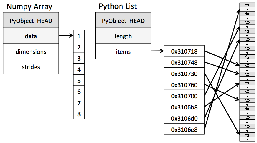
本章将详细介绍NumPy。 NumPy(Numerical Python的缩写)提供了一个有效的接口来存储和操作密集数据缓冲区。在某些方面,NumPy数组就像Python的内置列表类型,但NumPy数组提供了更高效的存储和数据操作,因为数组的大小越来越大。NumPy数组构成了Python中几乎整个数据科学工具生态系统的核心,因此无论数据科学的哪些方面感兴趣,学习有效使用NumPy的时间都是有价值的。
如果您按照前言中列出的建议并安装了Anaconda堆栈,那么您已经安装了NumPy并准备好了。如果您更喜欢自己动手类型,可以访问http://www.numpy.org/并按照其中的安装说明进行操作。完成后,您可以导入NumPy并仔细检查版本:
In [1]: import numpy

In [2]: numpy.__version__
Out[2]: '1.16.2'
对于这里讨论的软件包,我建议使用NumPy 1.8或更高版本。按照惯例,您会发现SciPy / PyData世界中的大多数人将使用np作为别名导入NumPy:
import numpy as np
在本章以及本书的其余部分中,您会发现这是我们导入和使用NumPy的方式。
在阅读本章时,不要忘记IPython使您能够快速浏览包的内容(通过使用制表符完成功能),以及各种功能的文档(使用?字符 - 请参阅IPython中的帮助和文档)。
例如,要显示numpy命名空间的所有内容,可以键入:
In [3]: np.<TAB>
要显示NumPy的内置文档,您可以使用:
In [4]: np?
有关更详细的文档以及教程和其他资源,请访问http://www.numpy.org
最近想爬点数据,但是之前的环境安装包的时候很随便。现在想养成良好的开发习惯,按项目来配置,所以理所当然的想到使用virtualenv。虚拟环境之前就创建好,但只是在命令行上使用,在PyCharm上使用的话能够更方便以后可视化的操作。
以下是操作步骤,配置还是比较简单的。
创建项目
打开PyCharm,依次点击File-New Project

配置虚拟环境

Create Project页面上,点击Location右侧设置项目的路径Porject Interpreter: Existing interpreter下拉菜单
New environment using:新建虚拟环境目录以及所用的解释器Existing Interpreter:选择已经创建好的虚拟环境点击Create即创建好使用虚拟环境的目录。

Terminal标签,提示符前出现虚拟环境名称即表示配置成功。PyCharm中可以配置运行不同的python文件使用不同的虚拟环境。
依次打开File-Settings-Project-Project Interpreter,点击Project Interpreter右侧的配置按钮,点Add。

在弹出窗口中点击Existing Interpreter,选择要添加的虚拟环境即可。如果想要在所有项目中生效,可勾选可选框。

添加成功后可以看到有多个虚拟环境

这时就可以根据实际的需要来配置运行python文件所用到的解释器


pgadmin4使用虚拟环境的作用在于将python应用开发环境与系统python完全隔离开来,它是系统python的一个副本,这样可以避免一些软件包出现版本冲突问题。如,A应用使用的是package 3.2+,而B应用只能使用package 2.9-,如果都使用系统环境就会造成冲突,使用虚拟环境后就可以避免这种情况。
python虚拟环境# 安装virtualenv(工作目录为/www/services/pgadmin4)
# 使用目标python版本的pip来安装
[root@gp6 services]# pip37 install virtualenv
# 创建虚拟环境时指定python版本
# 由于系统存在多个python版本,且virtualenv的路径没添加以PATH中,需以绝对路径创建
# 其中python3.7安装的virtualenv路径为/usr/local/python3.7/bin/virtualenv
[root@gp6 services]# /usr/local/python3.7/bin/virtualenv -p /usr/bin/python37 pgadmin4
# 使用系统python直接创建
# virtualenv pgadmin4
注意:若没指定虚拟环境的目录,会在当前工作环境创建一个与虚拟环境相同的目录。
# 注意:激活后命令提示符前会带(pgadmin4)字样
[root@gp6 services]# cd pgadmin4
[root@gp6 pgadmin4]# . ./bin/activate
(pgadmin4) [root@gp6 pgadmin4]#
deactivate
pgadmin4pgadmin4postgre官网下载最新的pgadmin4安装包,安装包已经包含所要的依赖包。#
(pgadmin4) [root@gp6 www]# cd /www/services
# 下载
(pgadmin4) [root@gp6 pgadmin4]# wget https://ftp.postgresql.org/pub/pgadmin/pgadmin4/v4.3/pip/pgadmin4-4.3-py2.py3-none-any.whl
pgadmin4所需要的依赖包如下:
python-flask-principal
python-flask-babel
python-flask
python-flask-wtf
python-flask-security
python-flask-gravatar
python-flask-mail
python-dateutil
django-htmlmin
babel
python-flask-login
python-wsgiref
python-fixtures
python-pbr
python-mimeparse
python-flask-sqlalchemy
python-pyrsistent
python-simplejson
python-wtforms
python-beautifulsoup4
python-itsdangerous
python-sqlalchemy
python-werkzeug
python-markupsafe
pytz
python-sqlparse
python-jinja2
pgadmin4# 激活虚拟环境后就安装pgadmin4
(pgadmin4) [root@gp6 pgadmin4]# pip install pgadmin4-4.3-py2.py3-none-any.whl
在虚拟环境中安装的包都会安装到./lib/python3.7/site-packages中
pgadmin4# 查出配置文件路径(进入虚拟环境目录 )
# find . -name "config.py"
# 拷贝配置文件
(pgadmin4) [root@gp6 pgadmin4]# cp ./lib/python3.7/site-packages/pgadmin4/config.py ./lib/python3.7/site-packages/pgadmin4/config_local.py
mkdir -p /www/services/pgadmin4/data/log
mkdir -p /www/services/pgadmin4/data/storage
mkdir -p /www/services/pgadmin4/data/sessions
(pgadmin4) [root@gp6 pgadmin4]# vi ./lib/python3.7/site-packages/pgadmin4/config_local.py

# 1. 修改服务器IP
# 将config_local.py里的“DEFAULT_SERVER = '127.0.0.1'”修改成服务器的IP。我机器修改如下:“DEFAULT_SERVER = '192.168.99.71'”

# 2. 配置pgAdmin的存储其会话数据,存储数据和日志:
LOG_FILE = '/www/services/pgadmin4/data/log/pgadmin4.log'
SQLITE_PATH = '/www/services/pgadmin4/data/pgadmin4.db'
SESSION_DB_PATH = '/www/services/pgadmin4/data/sessions'
STORAGE_DIR = '/www/services/pgadmin4/data/storage'
SERVER_MODE = True
以下是这五个指令的作用:
LOG_FILE:这定义了将存储pgAdmin日志的文件。
SQLITE_PATH:pgAdmin将用户相关数据存储在SQLite数据库中,该指令将pgAdmin软件指向此配置数据库。由于此文件位于持久目录/www/services/pgadmin4/data/下,因此升级后您的用户数据不会丢失。
SESSION_DB_PATH:指定将用于存储会话数据的目录。
STORAGE_DIR:定义pgAdmin将存储其他数据的位置,例如备份和安全证书。
SERVER_MODE:设置此指令以True告知pgAdmin在服务器模式下运行,而不是桌面模式。
(pgadmin4) [root@gp6 pgadmin4]# python ./lib/python3.7/site-packages/pgadmin4/setup.py
pgadmin4# 找出pgAdmin4.py的路径
(pgadmin4) [root@gp6 pgadmin4]# find . -name "pgAdmin4.py"
./lib/python3.7/site-packages/pgadmin4/pgAdmin4.py
# 在终端运行pgadmin4后,会显示网页访问的访问方式 ip:port
(pgadmin4) [root@gp6 pgadmin4]# python ./lib/python3.7/site-packages/pgadmin4/pgAdmin4.py
/www/services/pgadmin4/lib/python3.7/site-packages/psycopg2/__init__.py:144: UserWarning: The psycopg2 wheel package will be renamed from release 2.8; in order to keep installing from binary please use "pip install psycopg2-binary" instead. For details see: <http://initd.org/psycopg/docs/install.html#binary-install-from-pypi>.
""")
Starting pgAdmin 4. Please navigate to http://192.168.99.71:5050 in your browser.
* Running on http://192.168.99.71:5050/ (Press CTRL+C to quit)
pgadmin4# 在浏览器上输入第5点中的ip:port,输入帐号密码就可以登录pgadmin4管理页面了。
使用lxml解释html代码时报了OSError: Error reading file;【网页内容】failed to load external entity的错误
    start_url = 'https://gz.lianjia.com/ershoufang/yuexiu/'
    content = requests.get(start_url).text
    s = etree.parse(content, etree.HTMLParser())
    district = s.xpath('/html/body/div[3]/div/div[1]/dl[2]/dd/div[1]/div/a/@href')
    print(district)
从提示信息可以得出是读取文件内容时错误。。。具体是什么原因开始从错误信息中无法得知。
然而如果将content的内容写到html文件时,该错误就不会产生。即
s = etree.parse('index.html', etree.HTMLParser())
在网上搜了很久才发现原来问题出在parse()的参数里。因为parse()的参数主要如下:
In concert with what mzjn said, if you do want to pass a string to etree.parse(), just wrap it in a StringIO object.
etree.parse(source) expects source to be one of
- a file name/path
- a file object
- a file-like object
- a URL using the HTTP or FTP protocol
To parse from a string, use the fromstring() function instead.
要解释字符串时可以使用fromstring
s = etree.fromstring(content, etree.HTMLParser())
或者使用StringIO包裹起来
s = etree.parse(StringIO(content), etree.HTMLParser())
看来还是经验不足导致解决问题的思路不清晰。遇到这样的问题时,应该第一时间查看下parse()的使用方法。如果这样的话就找到是参数问题了。
今天在学习Scrapy 入门教程这文章时,在win10上运行以下代码报TypeError: write() argument must be str, not bytes错误。
def parse(self, response):
    filename = "teacher.html"
    open(filename, 'w').write(response.body)
从错误提示可知,因为传入write()函数的是bytes,而它要求是str。开始我没注意,所以走了很多弯路。修改成以下后,上面问题解决了。
def parse(self, response):
    filename = "teacher.html"
    open(filename, 'wb').write(response.body)
然而我打开下载后的文件发现编码为UTF-8-BOM,而之前验证网页编码(print(response.encoding))时发现是UTF-8。这差异就引起我的好奇心,因为以前学习时那些教程都说不要保存成带BOM的,所以就想将网页内容保存成UTF-8。

尝试将response.body转成utf-8时,抛出的错误提示是UnicodeEncodeError: 'gbk' codec can't encode character '\ufeff' in position 0: illegal multibyte sequence。
def parse(self, response):
    filename = "teacher.html"
    open(filename, 'w').write(response.body.decode('utf-8'))
查了下\ufeff这个字符是byte order mark,也就是BOM,所以保存的文件编码会是UTF-8-BOM。但是出现的gbk又引起我的注意。尝试直接转成gbk后,又抛出了UnicodeDecodeError: 'gbk' codec can't decode byte 0xbf in position 2: illegal multibyte sequence这错误提示。搜索0xbf发现这是UTF-8-BOM文件开头三个字符之一:0xEF 0xBB 0xBF。而\ufeff就是0xEF 0xBB 0xBF的UTF-8字符。

搜了下scrapy utf-8-bom转utf-8,发现网上都说直接保存网页内容都是utf-8-bom的。最终修改成以下代码,终于可以将文件保存成UTF-8了。
def parse(self, response):
    filename = "teacher.html"
    open(filename, 'wb').write(response.body.decode('UTF-8-sig').replace(u'\xa0', u' ').encode('utf-8'))
虽然将utf-8-bom转utf-8只是强迫症发作的行为。但好处是加深了对BOM的了解,以及Scrapy直接保存网页内容时的编码问题。不过linux系统下是否也是同样的情况留待以后再验证啦。
Pandas对象介绍在最基本的层面上,Pandas对象可以被认为是NumPy结构化数组的增强版本,其中行和列用标签而不是简单的整数索引来标识。正如我们将在本章的中看到的那样,Pandas在基本数据结构之上提供了许多有用的工具,方法和功能,但几乎所有后续内容都需要了解这些结构是什么。因此,在我们进一步讨论之前,让我们介绍这三个基本的Pandas数据结构:Series,DataFrame和Index。
我们将使用标准的NumPy和Pandas导入开始我们的代码会话:
In [1]: import numpy as np
   ...: import pandas as pd
Pandas Series对象Pandas Series是索引数据的一维数组。它可以从列表或数组创建,如下所示:
In [2]: data = pd.Series([0.25, 0.5, 0.75, 1.0])
   ...: data
Out[2]:
0    0.25
1    0.50
2    0.75
3    1.00
dtype: float64
正如我们在输出中看到的那样,Series包含了一系列值和一系列索引,我们可以使用values和index属性来访问它们。这些值只是一个熟悉的NumPy数组:
In [3]: data.values
Out[3]: array([0.25, 0.5 , 0.75, 1.  ])
索引是类型为pd.Index的类数组对象,我们将在稍后详细讨论。
In [4]: data.index
Out[4]: RangeIndex(start=0, stop=4, step=1)
与NumPy数组一样,通过熟悉的Python方括号表示法相关的索引可以访问数据:
In [5]: data[1]
Out[5]: 0.5

In [6]: data[1:3]
Out[6]:
1    0.50
2    0.75
dtype: float64
正如我们将要看到的,Pandas Series比它模拟的一维NumPy阵列更加通用和灵活。
NumPy数组的Series从我们目前所看到的情况来看,看起来Series对象基本上可以与一维NumPy数组互换。本质区别在于索引的存在:虽然Numpy数组具有用于访问值的隐式定义的整数索引,但Pandas Series具有与值相关联的显式定义的索引。
此显式索引定义为Series对象提供了其他功能。例如,索引不必是整数,但可以包含任何所需类型的值。例如,如果我们愿意,我们可以使用字符串作为索引:
In [7]: data = pd.Series([0.25, 0.5, 0.75, 1.0],
   ...:                  index=['a', 'b', 'c', 'd'])
   ...: data
Out[7]:
a    0.25
b    0.50
c    0.75
d    1.00
dtype: float64
可按预期来访问数据项:
In [8]: data['b']
Out[8]: 0.5
我们甚至可以使用非连续或非有续的索引:
In [9]: data = pd.Series([0.25, 0.5, 0.75, 1.0],
   ...:                  index=[2, 5, 3, 7])
   ...: data
Out[9]:
2    0.25
5    0.50
3    0.75
7    1.00
dtype: float64

In [10]: data[5]
Out[10]: 0.5
Series作为特定的字典通过这种方式,您可以将Pandas Series看作有点像Python字典的特化。字典是将任意键映射到一组任意值的结构,而Series是将任意键值映射到一组任意值的结构。这种类型很重要:正如NumPy数组背后的特定类型的编译代码使得它在特定操作上比Python列表更高效,Pandas Series的类型信息使得它在某些操作上比Python字典更高效。
通过直接从Python字典构造Series对象,可以使Series-as-dictionary类比更加清晰:
In [11]: population_dict = {'California': 38332521,
    ...:                    'Texas': 26448193,
    ...:                    'New York': 19651127,
    ...:                    'Florida': 19552860,
    ...:                    'Illinois': 12882135}
    ...: population = pd.Series(population_dict)
    ...: population
Out[11]:
California    38332521
Texas         26448193
New York      19651127
Florida       19552860
Illinois      12882135
dtype: int64
默认情况下,Series从有序键值的索引来创建的。从这里,可以执行典型的字典式项目访问:
In [12]: population['California']
Out[12]: 38332521
但是,与字典不同,Series还支持数组样式的操作,例如切片:
In [13]: population['California':'Illinois']
Out[13]:
California    38332521
Texas         26448193
New York      19651127
Florida       19552860
Illinois      12882135
dtype: int64
我们将讨论数据索引和选择中Pandas索引和切片的一些技巧。
我们已经看到了从头开始构建Pandas Series的几种方法;所有这些都是以下版本的某些版本:
>>> pd.Series(data, index=index)
其中index是可选参数,数据可以是许多实体之一。 例如,数据可以是列表或NumPy数组,在这种情况下,索引默认为整数序列:
In [15]: pd.Series([2, 4, 6])
Out[15]:
0    2
1    4
2    6
dtype: int64
数据可以是标量,重复填充指定的索引:
In [16]: pd.Series(5, index=[100, 200, 300])
Out[16]:
100    5
200    5
300    5
dtype: int64
data可以是字典,其中index默认为已排序的字典键:
In [17]: pd.Series({2:'a', 1:'b', 3:'c'})
Out[17]:
2    a
1    b
3    c
dtype: object
在每种情况下,如果首选不同的结果,则可以显式设置索引:
In [18]: pd.Series({2:'a', 1:'b', 3:'c'}, index=[3, 2])
Out[18]:
3    c
2    a
dtype: object
请注意,在这种情况下,Series仅使用明确标识的键填充。
Pandas DataFrame对象Pandas的下一个基本结构是DataFrame。与上一节中讨论的Series对象一样,DataFrame既可以被认为是NumPy数组的泛化,也可以被认为是Python字典的特化。我们现在来看看这些观点。
DataFrame作为通用的NumPy数组如果Series是具有灵活索引的一维数组的模拟,则DataFrame是具有灵活行索引和灵活列名称的二维数组的模拟。正如您可能将二维数组视为对齐的一维列的有序序列一样,您可以将DataFrame视为一系列对齐的Series对象。在这里,“对齐”是指它们共享相同的索引。
为了证明这一点,我们首先构建一个新Series,列出上一节中讨论的五个状态中每个状态的区域:
In [19]: area_dict = {'California': 423967, 'Texas': 695662, 'New York': 141297,
    ...:              'Florida': 170312, 'Illinois': 149995}
    ...: area = pd.Series(area_dict)
    ...: area
Out[19]:
California    423967
Texas         695662
New York      141297
Florida       170312
Illinois      149995
dtype: int64
现在我们已经将它与之前的种群Series一起使用,我们可以使用字典来构造包含此信息的单个二维对象:
In [20]: states = pd.DataFrame({'population': population,
    ...:                        'area': area})
    ...: states
Out[20]:
            population    area
California    38332521  423967
Texas         26448193  695662
New York      19651127  141297
Florida       19552860  170312
Illinois      12882135  149995
与Series对象一样,DataFrame有一个index属性,可以访问索引标签:
In [21]: states.index
Out[21]: Index(['California', 'Texas', 'New York', 'Florida', 'Illinois'], dtype='object')
此外,DataFrame有一个columns属性,它是一个包含列标签的Index对象:
In [22]: states.columns
Out[22]: Index(['population', 'area'], dtype='object')
因此,DataFrame可以被认为是二维NumPy数组的一般化,其中行和列都具有用于访问数据的通用索引。
DataFrame作为字典特例同样,我们也可以将DataFrame视为字典的特例。在字典将键映射到值的情况下,DataFrame将列名映射到一系列列数据。例如,要求'area'属性返回包含我们之前看到的区域的Series对象:
In [23]: states['area']
Out[23]:
California    423967
Texas         695662
New York      141297
Florida       170312
Illinois      149995
Name: area, dtype: int64
注意这里潜在的混淆点:在一个二维NumPy数组中,data [0]将返回第一行。对于DataFrame,data ['col0']将返回第一列。因此,将DataFrames视为通用字典而不是通用数组可能更好,尽管两种方式都可以查看情况。我们将探索在数据索引和选择中索引DataFrames的更灵活方法。
DataFrame对象Pandas DataFrame可以以多种方式构建。这里我们举几个例子。
Series对象DataFrame是Series对象的集合,单列DataFrame可以从单个Series中构建:
In [24]: pd.DataFrame(population, columns=['population'])
Out[24]:
            population
California    38332521
Texas         26448193
New York      19651127
Florida       19552860
Illinois      12882135
任何字典列表都可以生成DataFrame。我们将使用简单的列表生成式来创建一些数据:
In [25]: data = [{'a': i, 'b': 2 * i}
    ...:         for i in range(3)]
    ...: pd.DataFrame(data)
Out[25]:
   a  b
0  0  0
1  1  2
2  2  4
即使字典中的某些键丢失,Pandas也会用NaN(即“非数字”)值填充它们:
In [26]: pd.DataFrame([{'a': 1, 'b': 2}, {'b': 3, 'c': 4}])
Out[26]:
     a  b    c
0  1.0  2  NaN
1  NaN  3  4.0
Series对象的字典正如我们之前看到的,DataFrame也可以从Series对象的字典构造:
In [27]: pd.DataFrame({'population': population,
    ...:               'area': area})
Out[27]:
            population    area
California    38332521  423967
Texas         26448193  695662
New York      19651127  141297
Florida       19552860  170312
Illinois      12882135  149995
NumPy数组给定二维数据数组,我们可以创建具有任何指定列和索引名称的DataFrame。如果省略,将为每个使用整数索引
In [28]: pd.DataFrame(np.random.rand(3, 2),
...: columns=['foo', 'bar'],
...: index=['a', 'b', 'c'])
Out[28]:
foo bar
a 0.975209 0.685941
b 0.370348 0.502609
c 0.521795 0.358374
NumPy结构化数组我们在结构化数据中介绍了结构化数组:NumPy的结构化数组。 Pandas DataFrame的运行方式与结构化数组非常相似,可以直接从一个数组创建:
In [29]: A = np.zeros(3, dtype=[('A', 'i8'), ('B', 'f8')])
...: A
Out[29]: array([(0, 0.), (0, 0.), (0, 0.)], dtype=[('A', '<i8'), ('B', '<f8')])
In [30]: pd.DataFrame(A)
Out[30]:
A B
0 0 0.0
1 0 0.0
2 0 0.0
Pandas索引对象我们在这里看到,Series和DataFrame对象都包含一个显式索引,可以引用和修改数据。这个Index对象本身就是一个有趣的结构,它可以被认为是一个不可变数组或一个有序集(技术上是一个多集,因为Index对象可能包含重复的值)。这些视图在Index对象上可用的操作中会产生一些有趣的结果。举个简单的例子,让我们从整数列表构造一个索引:
In [31]: ind = pd.Index([2, 3, 5, 7, 11])
...: ind
Out[31]: Int64Index([2, 3, 5, 7, 11], dtype='int64')
索引在很多方面都像数组一样操作。例如,我们可以使用标准的Python索引表示法来检索值或切片:
In [32]: ind[1]
Out[32]: 3
In [33]: ind[::2]
Out[33]: Int64Index([2, 5, 11], dtype='int64')
索引对象还具有许多NumPy数组中熟悉的属性:
In [34]: print(ind.size, ind.shape, ind.ndim, ind.dtype)
5 (5,) 1 int64
Index对象和NumPy数组之间的一个区别是索引是不可变的 - 也就是说,它们不能通过常规方式修改:
In [35]: ind[1] = 0
---------------------------------------------------------------------------
TypeError Traceback (most recent call last)
<ipython-input-35-906a9fa1424c> in <module>
----> 1 ind[1] = 0
e:\dev\env\data\lib\site-packages\pandas\core\indexes\base.py in __setitem__(self, key, value)
3935
3936 def __setitem__(self, key, value):
-> 3937 raise TypeError("Index does not support mutable operations")
3938
3939 def __getitem__(self, key):
TypeError: Index does not support mutable operations
这种不变性使得在多个DataFrame和数组之间共享索引更安全,而不会由于无意的索引修改而产生副作用。
Pandas对象旨在促进跨数据集的连接等操作,这取决于集合算法的许多方面。Index对象遵循Python内置集合数据结构使用的许多约定,因此可以以熟悉的方式计算联合,交集,差异和其他组合:
In [36]: indA = pd.Index([1, 3, 5, 7, 9])
...: indB = pd.Index([2, 3, 5, 7, 11])
In [37]: indA & indB # intersection
Out[37]: Int64Index([3, 5, 7], dtype='int64')
In [38]: indA | indB # union
Out[38]: Int64Index([1, 2, 3, 5, 7, 9, 11], dtype='int64')
In [39]: indA ^ indB # symmetric difference
Out[39]: Int64Index([1, 2, 9, 11], dtype='int64')
也可以通过对象方法访问这些操作,例如indA.intersection(indB)。
NumPy的结构化数组虽然我们的数据通常可以通过同类数组来很好地表示,但有时并非如此。本节演示了NumPy结构化数组和记录数组的使用,它们为复合异构数据提供了有效的存储。虽然此处显示的模式对于简单操作很有用,但像这样的场景通常适合使用Pandas Dataframes,我们将在第3章中探讨。
In [1]: import numpy as np
想象一下,我们在很多人身上都有几类数据(比如姓名,年龄和体重),我们希望存储这些值以便在Python程序中使用。可以将它们存储在三个独立的数组中:
In [2]: name = ['Alice', 'Bob', 'Cathy', 'Doug']
...: age = [25, 45, 37, 19]
...: weight = [55.0, 85.5, 68.0, 61.5]
但这有点笨拙。这里没有任何东西可以告诉我们三个数组是相关的;如果我们可以使用单一结构来存储所有这些数据,那将更自然。NumPy可以通过结构化数组处理这个问题,结构化数组是具有复合数据类型的数组。
In [3]: x = np.zeros(4, dtype=int)
我们可以使用复合数据类型规范类似地创建结构化数组:
In [4]: # Use a compound data type for structured arrays
...: data = np.zeros(4, dtype={'names':('name', 'age', 'weight'),
...: 'formats':('U10', 'i4', 'f8')})
...: print(data.dtype)
[('name', '<U10'), ('age', '<i4'), ('weight', '<f8')]
这里'U10'转换为“最大长度为10的Unicode字符串”,“i4”转换为“4字节(即32位)整数”,“f8”转换为“8字节(即64位)浮点数“。我们将在下一节中讨论这些类型代码的其他选项。
现在我们已经创建了一个空容器数组,我们可以使用我们的值列表填充数组:
In [5]: data['name'] = name
...: data['age'] = age
...: data['weight'] = weight
...: print(data)
[('Alice', 25, 55. ) ('Bob', 45, 85.5) ('Cathy', 37, 68. )
('Doug', 19, 61.5)]
正如我们所希望的那样,数据现在被安排在一个方便的内存块中。
结构化数组的便利之处在于您现在可以通过索引或名称来引用值:
In [6]: # Get all names
...: data['name']
Out[6]: array(['Alice', 'Bob', 'Cathy', 'Doug'], dtype='<U10')
In [7]: # Get first row of data
...: data[0]
Out[7]: ('Alice', 25, 55.)
In [8]: # Get the name from the last row
...: data[-1]['name']
Out[8]: 'Doug'
使用布尔掩码,这甚至允许您执行一些更复杂的操作,例如过滤年龄:
In [9]: # Get names where age is under 30
...: data[data['age'] < 30]['name']
Out[9]: array(['Alice', 'Doug'], dtype='<U10')
请注意,如果您想进行任何比这些更复杂的操作,您应该考虑下一章中介绍的Pandas包。正如我们将看到的,Pandas提供了一个Dataframe对象,它是一个构建在NumPy数组上的结构,它提供了各种有用的数据操作功能,类似于我们在这里展示的功能,以及更多。
可以通过多种方式指定结构化数组数据类型。之前,我们看过字典方法:
In [10]: np.dtype({'names':('name', 'age', 'weight'),
...: 'formats':('U10', 'i4', 'f8')})
Out[10]: dtype([('name', '<U10'), ('age', '<i4'), ('weight', '<f8')])
为清楚起见,可以使用Python类型或NumPy dtypes指定数字类型:
In [11]: np.dtype({'names':('name', 'age', 'weight'),
...: 'formats':((np.str_, 10), int, np.float32)})
Out[11]: dtype([('name', '<U10'), ('age', '<i4'), ('weight', '<f4')])
复合类型也可以指定为元组列表:
In [12]: np.dtype([('name', 'S10'), ('age', 'i4'), ('weight', 'f8')])
Out[12]: dtype([('name', 'S10'), ('age', '<i4'), ('weight', '<f8')])
如果类型的名称对您无关紧要,则可以在逗号分隔的字符串中单独指定类型:
In [13]: np.dtype('S10,i4,f8')
Out[13]: dtype([('f0', 'S10'), ('f1', '<i4'), ('f2', '<f8')])
缩短的字符串格式代码可能看起来令人困惑,但它们建立在简单的规则之上。第一个(可选)字符是<或>,分别表示“little endian”或“big endian”,并指定有效位的排序约定。下一个字符指定数据类型:字符,字节,整数,浮点等(参见下表)。最后一个或多个字符表示对象的大小(以字节为单位)。
| Character | Description | Example |
|---|---|---|
| 'b' | Byte | np.dtype('b') |
| 'i' | Signed integer | np.dtype('i4') == np.int32 |
| 'u' | Unsigned integer | np.dtype('u1') == np.uint8 |
| 'f' | Floating point | np.dtype('f8') == np.int64 |
| 'c' | Complex floating point | np.dtype('c16') == np.complex128 |
| 'S', 'a' | String | np.dtype('S5') |
| 'U' | Unicode string | np.dtype('U') == np.str_ |
| 'V' | Raw data (void) | np.dtype('V') == np.void |
可以定义更高级的化合物类型。例如,您可以创建一个类型,其中每个元素包含一个数组或值矩阵。在这里,我们将创建一个数据类型,其中mat组件由3×3浮点矩阵组成:
In [14]: tp = np.dtype([('id', 'i8'), ('mat', 'f8', (3, 3))])
...: X = np.zeros(1, dtype=tp)
...: print(X[0])
...: print(X['mat'][0])
(0, [[0., 0., 0.], [0., 0., 0.], [0., 0., 0.]])
[[0. 0. 0.]
[0. 0. 0.]
[0. 0. 0.]]
现在,X数组中的每个元素都包含一个id和一个3×3矩阵。为什么要使用它而不是简单的多维数组,或者Python字典呢?原因是这个NumPy dtype直接映射到C结构定义,因此包含数组内容的缓冲区可以在适当编写的C程序中直接访问。如果您发现自己正在为操作结构化数据的遗留C或Fortran库编写Python接口,您可能会发现结构化数组非常有用!
RecordArrays:具有Twist的结构化数组NumPy还提供了np.recarray类,它几乎与刚刚描述的结构化数组相同,但还有一个附加功能:字段可以作为属性而不是字典键来访问。回想一下,我们以前写过:
In [15]: data['age']
Out[15]: array([25, 45, 37, 19])
如果我们将数据视为记录数组,我们可以通过少量击键来访问它:
In [16]: data_rec = data.view(np.recarray)
...: data_rec.age
Out[16]: array([25, 45, 37, 19])
缺点是对于记录数组,即使使用相同的语法,访问字段也会涉及一些额外的开销。我们在这里可以看到:
In [17]: %timeit data['age']
...: %timeit data_rec['age']
...: %timeit data_rec.age
133 ns ± 11.4 ns per loop (mean ± std. dev. of 7 runs, 10000000 loops each)
3.83 µs ± 256 ns per loop (mean ± std. dev. of 7 runs, 100000 loops each)
5.19 µs ± 477 ns per loop (mean ± std. dev. of 7 runs, 100000 loops each)
更方便的符号是否值得额外开销将取决于您自己的应用程序。
On to Pandas关于结构化和记录数组的这一部分是故意在本章的最后部分,因为它很好地介绍了我们将要介绍的下一个包:Pandas。像这里讨论的结构化数组在某些情况下很容易了解,特别是在您使用NumPy数组映射到C,Fortran或其他语言的二进制数据格式的情况下。对于结构化数据的日常使用,Pandas包是一个更好的选择,我们将在下一章中深入讨论它。
# coding: utf-8
#
import pandas as pd
def category_datas(filepath):
# ExcelFile对象
excelFile = pd.ExcelFile(filepath)
# sheet列表
sheet_names = excelFile.sheet_names[2:]
# 日期
trade_datas = pd.DataFrame([], columns=['品类', '日期', '分公司', '系数', '交易金额'])
for i in range(len(sheet_names)):
# 品类名称
category = sheet_names[i]
# 读取sheet的数据
df = pd.read_excel(excelFile, category)
rows = len(df.index) - 1
cat_list = [category] * rows
category = pd.DataFrame(cat_list,columns=['品类'])
# 分公司,重置索引
sub_company = df.iloc[1:,0].reset_index(drop=True).to_frame()
# 系数 #
ratio = df.iloc[1:,1].reset_index(drop=True)
ratio.name = '系数'
ratio = ratio.to_frame()
# 日期、交易金额#
# 数据日期
dates = list(df.columns[2:-1])
#
for idx in range(len(dates)):
#
date = dates[idx]
data_list = [date] * rows
data_date = pd.DataFrame(data_list,columns=['日期'])
# 交易金额
id = idx + 2
trade_amt = df.iloc[1:, id].reset_index(drop=True)
trade_amt.name = '交易金额'
trade_amt = trade_amt.to_frame()
# 合并各指标
trade_data = pd.concat([category, data_date, sub_company, ratio, trade_amt], axis = 1)
# 合并
trade_datas = trade_datas.append(trade_data).reset_index(drop=True)
return trade_datas
# def main():
filepath = './data/20181208_trade_amt_1201-1214.xlsx'
trade_datas = category_datas(filepath)
trade_datas.to_excel('./data/20181208_trade_amt_1201-1214(处理).xlsx', index=False)我们在上一节中看到NumPy的通用函数如何用于向量化操作,从而消除慢速的Python循环。矢量化操作的另一种方法是使用NumPy的广播功能。广播只是用于在不同大小的阵列上应用二进制ufunc(例如,加法,减法,乘法等)的一组规则。
回想一下,对于相同大小的数组,二元操作是在逐个元素的基础上执行的:
In [1]: import numpy as np
In [2]: a = np.array([0, 1, 2])
...: b = np.array([5, 5, 5])
...: a + b
Out[2]: array([5, 6, 7])
广播允许在不同大小的数组上执行这些类型的二进制操作 - 例如,我们可以轻松地使数组与标量相加(将其视为0维数组):
In [3]: a + 5
Out[3]: array([5, 6, 7])
我们可以将此视为将值5拉伸或复制到数组[5,5,5]中并添加结果的操作。NumPy广播的优势在于,这种复制值实际上并没有发生,但是当我们考虑广播时,它是一种有用的心理模型。
我们可以类似地将其扩展到更高维度的数组。当我们将一维数组添加到二维数组时观察结果:
In [4]: M = np.ones((3, 3))
...: M
Out[4]:
array([[1., 1., 1.],
[1., 1., 1.],
[1., 1., 1.]])
In [5]: M + a
Out[5]:
array([[1., 2., 3.],
[1., 2., 3.],
[1., 2., 3.]])
这里,一维数组a被拉伸,或者在第二维上广播,以匹配M的形状。
虽然这些示例相对容易理解,但更复杂的情况可能涉及两个阵列的广播。请考虑以下示例:
In [6]: a = np.arange(3)
...: b = np.arange(3)[:, np.newaxis]
...:
...: print(a)
...: print(b)
[0 1 2]
[[0]
[1]
[2]]
In [7]: a + b
Out[7]:
array([[0, 1, 2],
[1, 2, 3],
[2, 3, 4]])
就像之前我们拉伸或广播一个值以匹配另一个的形状一样,这里我们已经拉伸了a和b以匹配一个共同的形状,结果是一个二维数组!这些示例的几何图形在下图中可视化(产生此图的代码可以在附录中找到,并根据astroML文档中发布的内容进行修改。经许可使用)。
浅色盒子代表广播的值:同样,这个额外的内存实际上并没有在操作过程中分配,但在概念上可以想象它是有用的。
NumPy中的广播遵循一套严格的规则来确定两个数组之间的交互:
1:如果两个阵列的尺寸数不同,则尺寸较小的阵列的形状(shape)将在其前(左)侧填充1。2:如果两个数组的形状(shape)在任何维度上都不匹配,则该维度中形状等于1的数组将被拉伸以匹配其他形状。3:如果在任何维度中,大小不一致且都不等于1,则会引发错误。为了明确这些规则,让我们详细考虑几个例子。
1让我们看一下将二维数组与一维数组相加:
In [8]: M = np.ones((2, 3))
...: a = np.arange(3)
让我们考虑对这两个数组进行操作。阵列的形状是
我们在规则1中看到数组a的维数较少,所以我们用左边的数据填充它:
根据规则2,我们现在看到第一个维度不同意,因此我们将此维度拉伸以匹配:
形状匹配,我们看到最终的形状将是(2,3):
In [9]: M + a
Out[9]:
array([[1., 2., 3.],
[1., 2., 3.]])
我们来看一个需要广播两个数组的例子:
In [10]: a = np.arange(3).reshape((3, 1))
...: b = np.arange(3)
同样,我们将首先写出数组的形状:
规则1说我们必须用b填充b的形状:
规则2告诉我们,我们升级这些中的每一个以匹配另一个数组的相应大小:
因为结果匹配,所以这些形状是兼容的。我们在这里可以看到:
In [11]: a + b
Out[11]:
array([[0, 1, 2],
[1, 2, 3],
[2, 3, 4]])
3现在让我们看一下两个数组不兼容的例子:
In [12]: M = np.ones((3, 2))
...: a = np.arange(3)
这与第一个例子中的情况略有不同:矩阵M被转置。这对计算有何影响?阵列的形状是
同样,规则1告诉我们必须填充a的形状:
根据规则2,a的第一个维度被拉伸以匹配M的维度:
现在我们点击规则3 - 最终的形状不匹配,所以这两个数组是不兼容的,我们可以通过尝试此操作来观察:
In [13]: M + a
---------------------------------------------------------------------------
ValueError Traceback (most recent call last)
<ipython-input-13-8cac1d547906> in <module>
----> 1 M + a
ValueError: operands could not be broadcast together with shapes (3,2) (3,)
注意这里可能存在的混淆:你可以想象通过在右边而不是左边填充一个形状来使a和M兼容。但这不是广播规则的工作方式!在某些情况下,这种灵活性可能会有用,但这会导致潜在的模糊区域。如果你想要右边填充,你可以通过重新整形数组来明确地执行此操作(我们将使用NumPy Arrays基础中引入的np.newaxis关键字):
In [14]: a[:, np.newaxis].shape
Out[14]: (3, 1)
In [15]: M + a[:, np.newaxis]
Out[15]:
array([[1., 1.],
[2., 2.],
[3., 3.]])
另请注意,虽然我们一直专注于+运算符,但这些广播规则适用于任何二元ufunc。例如,这里是logaddexp(a,b)函数,它比原始方法更精确地计算log(exp(a)+ exp(b)):
In [16]: np.logaddexp(M, a[:, np.newaxis])
Out[16]:
array([[1.31326169, 1.31326169],
[1.69314718, 1.69314718],
[2.31326169, 2.31326169]])
有关许多可用通用函数的更多信息,请参阅NumPy数组计算:通用函数。
广播操作构成了我们将在本书中看到的许多例子的核心。我们现在来看一些它们可能有用的简单示例。
在上一节中,我们看到ufuncs允许NumPy用户不再需要显式编写慢速Python循环。广播扩展了这种能力。一个常见的例子是使数组数据居中。想象一下,你有一个包含10个观测值的数组,每个观测值包含3个值。使用标准约定(参见Scikit-Learn中的数据表示),我们将其存储在10×3阵列中:
In [17]: X = np.random.random((10, 3))
我们可以使用第一维上的平均聚合来计算每个要素的平均值:
In [18]: Xmean = X.mean(0)
...: Xmean
Out[18]: array([0.44645094, 0.54261367, 0.56561384])
现在我们可以通过减去均值来中心X数组(这是一个广播操作):
In [19]: X_centered = X - Xmean
要仔细检查我们是否已正确完成此操作,我们可以检查居中数组是否接近零均值:
In [20]: X_centered.mean(0)
Out[20]: array([ 7.77156117e-17, -6.66133815e-17, -9.99200722e-17])
在机器精度范围内,平均值现在为0。
广播非常有用的一个地方是基于二维功能显示图像。如果我们想要定义一个函数z = f(x,y), z = f(x,y),广播可用于计算网格中的函数:
In [21]: # x and y have 50 steps from 0 to 5
...: x = np.linspace(0, 5, 50)
...: y = np.linspace(0, 5, 50)[:, np.newaxis]
...:
...: z = np.sin(x) ** 10 + np.cos(10 + y * x) * np.cos(x)
我们将使用Matplotlib绘制这个二维数组(这些工具将在密度和轮廓图中完整讨论):
In [22]: %matplotlib inline
...: import matplotlib.pyplot as plt
In [23]: plt.imshow(z, origin='lower', extent=[0, 5, 0, 5],
...: cmap='viridis')
...: plt.colorbar();
结果是二维函数的引人注目的可视化。
为了查阅朋友撤回的微信消息,我上网看了一些教程。参考Python查看微信好友撤回的消息 此贴的脚本来开发自己的脚本。但是使用过程中发现一些问题:
None对象来的None对象问题后,又出现以下问题,上网找了下答案没发现有解决方法。
Linux系统下需要设置enableCmdQR=2才能完全显示二围码。import re
import os
import time
import itchat
import platform
from itchat.content import TEXT
from itchat.content import *
msg_info = {}
face_package = None
# 处理接收到的信息
@itchat.msg_register([TEXT, PICTURE, FRIENDS, CARD, MAP, SHARING, RECORDING, ATTACHMENT, VIDEO], isFriendChat=True)
def handleRMsg(msg):
global face_package
# 指定用户列表
user_list = ['A', 'B', 'C']
# 接收消息的时间
msg_time_receive = time.strftime("%Y-%m-%d %H:%M:%S", time.localtime())
# 发信人
try:
msg_from = itchat.search_friends(userName=msg['FromUserName'])['NickName']
except:
msg_from = 'WeChat Official Accounts'
# 发信时间
msg_time_send = time.strftime("%Y-%m-%d %H:%M:%S", time.localtime(msg['CreateTime']))
# 信息ID
msg_id = msg['MsgId']
msg_content = None
msg_link = None
# 文本或者好友推荐
if msg['Type'] == 'Text' or msg['Type'] == 'Friends':
msg_content = msg['Text']
print('[Text/Friends]:【%s】%s:%s' % (msg_time_receive, msg_from, msg_content))
# 附件/视频/图片/语音
elif msg['Type'] == 'Attachment' or msg['Type'] == "Video" or msg['Type'] == 'Picture' or msg['Type'] == 'Recording':
msg_content = msg['FileName']
# 指定用户才下载文件
if msg_from in user_list:
msg['Text'](str(msg_content))
print('[Attachment/Video/Picture/Recording]: 【%s】%s:%s' % (msg_time_receive, msg_from, msg_content))
# 推荐名片
elif msg['Type'] == 'Card':
msg_content = msg['RecommendInfo']['NickName'] + '的推荐名片,'
if msg['RecommendInfo']['Sex'] == 1:
msg_content += '性别男。'
else:
msg_content += '性别女。'
print('[Card]:【%s】%s:%s' % (msg_time_receive, msg_from, msg_content))
# 位置信息
elif msg['Type'] == 'Map':
x, y, location = re.search("<location x=\"(.*?)\" y=\"(.*?)\".*label=\"(.*?)\".*", msg['OriContent']).group(1, 2, 3)
if location is None:
msg_content = r"纬度:" + x.__str__() + ", 经度:" + y.__str__()
else:
msg_content = r"" + location
print('[Map]:【%s】%s:%s' % (msg_time_receive, msg_from, msg_content))
# 分析的音乐/文章
elif msg['Type'] == 'Sharing':
msg_content = msg['Text']
msg_link = msg['Url']
print('[Sharing]:【%s】%s:%s' % (msg_time_receive, msg_from, msg_content))
msg_info.update(
{
msg_id: {
"msg_from": msg_from,
"msg_time_send": msg_time_send,
"msg_time_receive": msg_time_receive,
"msg_type": msg["Type"],
"msg_content": msg_content,
"msg_link": msg_link
}
}
)
face_package = msg_content
# 监听是否有消息撤回
@itchat.msg_register(NOTE, isFriendChat=True)
def monitor(msg):
if '撤回了一条消息' in msg['Content'] or 'recalled a message' in msg['Content'] :
recall_msg_id = re.search("\<msgid\>(.*?)\<\/msgid\>", msg['Content']).group(1)
recall_msg = msg_info.get(recall_msg_id)
if not recall_msg:
msg_from = itchat.search_friends(userName=msg['FromUserName'])['NickName']
msg_time_receive = time.strftime("%Y-%m-%d %H:%M:%S", time.localtime(msg['CreateTime']))
msg_prime = '【' + msg_from + '撤回了一条消息】 时间:' + msg_time_receive + ' 内容:' + face_package
itchat.send_msg(msg_prime, toUserName='filehelper')
print('[NoneType]: %s' % (msg_prime))
else:
print('[Recall]: %s' % recall_msg)
# 表情包:有时返回表情,msgid为小于11位的整数,此时recall_msg为NoneType,此时face_package保存着上一条接收到的信息的文件名
if len(recall_msg_id) < 11:
itchat.send_file(face_package, toUserName='filehelper')
elif recall_msg:
msg_prime = '【' + recall_msg.get('msg_from') + '撤回了一条消息】\n' \
'消息类型:' + recall_msg.get('msg_type') + '\n' \
'时间:' + recall_msg.get('msg_time_receive') + '\n' \
r'内容:' + recall_msg.get('msg_content')
if recall_msg['msg_type'] == 'Sharing':
msg_prime += '\n链接:' + recall_msg.get('msg_link')
itchat.send_msg(msg_prime, toUserName='filehelper')
if recall_msg['msg_type'] == 'Attachment' or recall_msg['msg_type'] == "Video" or recall_msg['msg_type'] == 'Picture' or recall_msg['msg_type'] == 'Recording':
file = '@fil@%s' % (recall_msg['msg_content'])
itchat.send(msg=file, toUserName='filehelper')
#try:
# # os.remove(recall_msg['msg_content'])
# print(recall_msg['msg_content'])
#except FileNotFoundError:
# # 删除文件失败时记录日志
# # os.remove(face_package)
# print('[NotFound]: %s' % recall_msg['msg_content'])
msg_info.pop(recall_msg_id)
if __name__ == '__main__':
if platform.platform()[:7] == 'Windows':
itchat.auto_login(enableCmdQR=False, hotReload=True)
else:
#itchat.auto_login(enableCmdQR=True, hotReload=True)
# linux下enableCmdQR传2才能显示完全
itchat.auto_login(enableCmdQR=2, hotReload=True)
itchat.run()每个Python对象都包含对字符串的引用,称为docstring,在大多数情况下,它将包含对象的简明摘要以及如何使用它。Python有一个内置的help()函数,可以访问这些信息并打印结果。例如,要查看内置len函数的文档,可以执行以下操作:
In [1]: help(len)
Help on built-in function len in module builtins:
len(obj, /)
Return the number of items in a container.
根据你的解释器,此信息可能会显示为内嵌文本,也可能显示在某个单独的弹出窗口中。
?访问文档因为查找对象的帮助是如此常见和有用,IPython引入了?字符作为访问此文档和其他相关信息的简写:
In [2]: len?
Signature: len(obj, /)
Docstring: Return the number of items in a container.
Type: builtin_function_or_method
这种表示法适用于任何对象,包括对象方法:
In [3]: L = [1 ,2 ,3]
In [4]: L.insert?
Docstring: L.insert(index, object) -- insert object before index
Type: builtin_function_or_method
甚至是对象本身,使用其类型的文档:
In [5]: L?
Type: list
String form: [1, 2, 3]
Length: 3
Docstring:
list() -> new empty list
list(iterable) -> new list initialized from iterable's items
重要的是,这甚至适用于您自己创建的功能或其他对象!在这里,我们将使用docstring定义一个小函数:
In [6]: def square(a):
...: """Return the square of a."""
...: return a ** 2
...:
请注意,要为我们的函数创建docstring,我们只需在第一行中放置一个字符串文字。因为docstring通常是多行,所以我们按照惯例使用Python的三重引号表示多行字符串。
在我们将使用?标记以查找此文档字符串:
In [7]: square?
Signature: square(a)
Docstring: Return the square of a.
File: c:\users\username\<ipython-input-6-3ed0e8c09915>
Type: function
通过docstrings快速访问文档是您应该养成始终在您编写的代码中添加此类内联文档的习惯的一个原因!
??访问源代码由于Python语言易于阅读,因此通常可以通过阅读您感兴趣的对象的源代码来获得另一层次的洞察力。 IPython提供了带有双重问号(??)的源代码的快捷方式:
In [8]: square??
Signature: square(a)
Source:
def square(a):
"""Return the square of a."""
return a ** 2
File: c:\users\username\<ipython-input-6-3ed0e8c09915>
Type: function
对于像这样的简单函数,双重问号可以快速了解内部的细节。
如果你玩这么多,你会注意到有时候??后缀不显示任何源代码:这通常是因为问题里的对象不是用Python实现的,而是用C语言或其他一些编译的扩展语言实现的。如果是这样的话,??后缀会给出与?相同的输出。你可以在许多Python的内置对象和类型中找到这种例外,例如上面的len:
In [9]: len??
Signature: len(obj, /)
Docstring: Return the number of items in a container.
Type: builtin_function_or_method
用?和/或??提供了一个强大而快速的界面,用于查找有关Python函数或模块的功能的信息。
Tab补全探索模块IPython的另一个有用的接口是使用tab键自动补全和探索对象,模块和名称空间的内容。在下面的示例中,我们将使用<TAB>指示何时应按Tab键
Tab补全对象内容每个Python对象都有各种与之关联的属性和方法。与前面讨论的help函数一样,Python有一个内置的dir函数,它返回这些函数的列表,但是tab-completion接口在实践中更容易使用。要查看对象的所有可用属性的列表,可以键入对象的名称,后跟句点(“.”)字符和Tab键:
In [10]: L.<TAB>
L.append L.count L.insert L.reverse
L.clear L.extend L.pop L.sort
L.copy L.index L.remove
要缩小列表范围,可以键入名称的第一个字符或多个字符,Tab键将找到匹配的属性和方法:
In [10]: L.co<TAB>
L.copy
L.count
如果只有一个选项,按Tab键将为您完成该行。例如,以下内容将立即替换为L.count:
In [10]: L.cou<TAB>
虽然Python没有严格强制区分公共/外部属性和私有/内部属性,但按照惯例,前面的下划线用于表示此类方法。为清楚起见,默认情况下会从列表中省略这些私有方法和特殊方法,但可以通过显式键入下划线来列出它们:
In [10]: L.__
L.__add__ L.__dir__ L.__getattribute__ L.__imul__ L.__len__
L.__class__ L.__doc__ L.__getitem__ L.__init__ L.__lt__
L.__contains__ L.__eq__ L.__gt__ L.__init_subclass__ L.__mul__
L.__delattr__ L.__format__ L.__hash__ L.__iter__ L.__ne__
L.__delitem__ L.__ge__ L.__iadd__ L.__le__ L.__new__
为简洁起见,我们只展示了输出的前几行。其中大多数是Python的特殊双下划线方法(通常昵称为“dunder”方法)。
Tab补全从包中导入对象时,Tab补全也很有用。在这里,我们将使用它来查找以co开头的itertools包中的所有可能的导入:
In [10]: from itertools import co<TAB>
combinations compress
combinations_with_replacement count
同样,您可以使用Tab补全来查看系统上可用的导入(这将根据Python会话可见的第三方脚本和模块而更改):
In [10]: import <TAB>
abc anaconda_navigator asn1crypto asyncio babel
adodbapi anaconda_project ast asyncore backports
afxres antigravity astroid atexit base64
aifc argparse astropy audioop bdb
alabaster array asynchat autoreload binascii
如果您知道要查找的对象或属性的前几个字符,则Tab补全很有用,但如果您想要匹配单词中间或末尾的字符,则很少有帮助。对于这种使用情况,IPython为使用*字符的名称提供了通配符匹配方法。
例如,我们可以使用它来列出命名空间中以Warning结尾的每个对象:
In [10]: *Warning?
BytesWarning
DeprecationWarning
FutureWarning
ImportWarning
PendingDeprecationWarning
ResourceWarning
RuntimeWarning
SyntaxWarning
UnicodeWarning
UserWarning
Warning
请注意,*字符匹配任何字符串,包括空字符串。
同样,假设我们正在寻找一个字符串方法,该方法在其名称中包含单词find。我们可以这样搜索:
In [12]: str.*find*?
str.find
str.rfind
我发现这种灵活的通配符搜索对于在了解新软件包或重新熟悉一个熟悉的软件包时查找特定命令非常有用。
注:以上代码的结果是在win10 pro的cmd窗口上输出的,跟文档里的有出入。
刚才看到pip提示有新版本,所以就手贱的升级了下
You are using pip version 19.0.2, however version 19.0.3 is available.
You should consider upgrading via the 'python -m pip install --upgrade pip' command.
(lianjia) e:\DEV\projects\spider>pip install -U pip
Collecting pip
Downloading https://files.pythonhosted.org/packages/d8/f3/413bab4ff08e1fc4828dfc59996d721917df8e8583ea85385d51125dceff/pip-19.0.3-py2.py3-none-any.whl (1.4MB)
100% |████████████████████████████████| 1.4MB 214kB/s
Installing collected packages: pip
Found existing installation: pip 19.0.2
Uninstalling pip-19.0.2:
Could not install packages due to an EnvironmentError: [WinError 5] 拒绝访问。: 'e:\\dev\\env\\lianjia\\scripts\\pip.exe'
Consider using the `--user` option or check the permissions.
由于我是在虚拟环境下执行的升级,所以就提示报权限问题。想安装其他包时提示pip不存在。
(lianjia) e:\DEV\projects\spider>pip install beautifulsoup4
Traceback (most recent call last):
File "d:\user\chenwj\apps\anaconda3\Lib\runpy.py", line 193, in _run_module_as_main
"__main__", mod_spec)
File "d:\user\chenwj\apps\anaconda3\Lib\runpy.py", line 85, in _run_code
exec(code, run_globals)
File "E:\DEV\env\lianjia\Scripts\pip.exe\__main__.py", line 5, in <module>
ModuleNotFoundError: No module named 'pip'
网上找了下不少人都遇到在windows下升级pip失败的案例。具体解决方法如下:
(lianjia) e:\DEV\projects\spider>curl https://bootstrap.pypa.io/get-pip.py -o get-pip.py
% Total % Received % Xferd Average Speed Time Time Time Current
Dload Upload Total Spent Left Speed
100 1659k 100 1659k 0 0 237k 0 0:00:07 0:00:07 --:--:-- 363k
(lianjia) e:\DEV\projects\spider>python get-pip.py
Collecting pip
Using cached https://files.pythonhosted.org/packages/d8/f3/413bab4ff08e1fc4828dfc59996d721917df8e8583ea85385d51125dceff/pip-19.0.3-py2.py3-none-any.whl
Installing collected packages: pip
Successfully installed pip-19.0.3
(lianjia) e:\DEV\projects\spider>pip -V
pip 19.0.3 from e:\dev\env\lianjia\lib\site-packages\pip (python 3.6)
通常,当面对大量数据时,第一步是计算相关数据的摘要统计数据。也许最常见的汇总统计数据是均值和标准差,它允许您汇总数据集中的“典型”值,但其他聚合也很有用(累加和,累积,中位数,最小值和最大值,分位数等。 )。
NumPy具有快速内置的聚合功能,可用于处理数组;我们将在这里讨论并演示其中的一些内容。
作为一个简单的示例,请考虑计算数组中所有值的总和。 Python本身可以使用内置的sum函数执行此操作:
In [1]: import numpy as np
In [2]: L = np.random.random(100)
...: sum(L)
...:
Out[2]: 50.19656740027611
语法与NumPy的sum函数非常相似,结果在最简单的情况下是相同的:
In [3]: np.sum(L)
Out[3]: 50.1965674002761
但是,因为它在编译代码中执行操作,所以NumPy的操作版本计算得更快:
In [4]: big_array = np.random.rand(1000000)
...: %timeit sum(big_array)
...: %timeit np.sum(big_array)
...:
74.8 ms ± 542 µs per loop (mean ± std. dev. of 7 runs, 10 loops each)
1.31 ms ± 64.4 µs per loop (mean ± std. dev. of 7 runs, 1000 loops each)
但要小心:sum函数和np.sum函数不相同,有时会导致混淆!特别是,它们的可选参数具有不同的含义,并且np.sum知道多个数组维度,我们将在下一节中看到。
类似地,Python具有内置的最小和最大函数,用于查找任何给定数组的最小值和最大值:
In [5]: min(big_array), max(big_array)
Out[5]: (5.128750490968059e-07, 0.9999988318220189)
NumPy的相应函数具有相似的语法,并且再次运行得更快:
In [7]: %timeit min(big_array)
...: %timeit np.min(big_array)
...:
59.2 ms ± 4.86 ms per loop (mean ± std. dev. of 7 runs, 10 loops each)
517 µs ± 20.4 µs per loop (mean ± std. dev. of 7 runs, 1000 loops each)
对于min,max,sum和其他几个NumPy聚合,更短的语法是使用数组对象本身的方法:
In [8]: print(big_array.min(), big_array.max(), big_array.sum())
5.128750490968059e-07 0.9999988318220189 499989.9197268303
只要有可能,请确保在NumPy数组上运行时使用这些聚合的NumPy版本!
一种常见类型的聚合操作是沿行或列的聚合。假设您有一些存储在二维数组中的数据:
In [9]: M = np.random.random((3, 4))
...: print(M)
...:
[[0.00728389 0.92617593 0.91146565 0.09980222]
[0.37296596 0.54088655 0.32771595 0.75633785]
[0.5521776 0.33464218 0.95525122 0.85253779]]
默认情况下,每个NumPy聚合函数将返回整个数组的聚合:
In [10]: M.sum()
Out[10]: 6.637242775730832
聚合函数采用另一个参数来指定计算聚合的轴。例如,我们可以通过指定axis = 0找到每列中的最小值:
In [11]: M.min(axis=0)
Out[11]: array([0.00728389, 0.33464218, 0.32771595, 0.09980222])
该函数返回四个值,对应于四列数字。 同样,我们可以找到每行中的最大值:
In [12]: M.max(axis=1)
Out[12]: array([0.92617593, 0.75633785, 0.95525122])
在此处指定轴的方式可能会使来自其他语言的用户感到困惑。 axis关键字指定将折叠的数组的维度,而不是将返回的维度。
因此,指定axis = 0意味着第一个轴将被折叠:对于二维数组,这意味着将聚合每列中的值。
NumPy提供了许多其他聚合函数,但我们不会在这里详细讨论它们。此外,大多数聚合都有一个NaN安全对应项,用于计算结果,同时忽略缺失值,缺失值由特殊的IEEE浮点NaN值标记(有关缺失数据的更全面讨论,请参阅处理缺失数据)。其中一些NaN安全功能直到NumPy 1.8才被添加,因此它们不适用于较旧的NumPy版本。
下表提供了NumPy中可用的有用聚合函数的列表:
Function Name |
NaN-safe Version |
Description |
|---|---|---|
np.sum |
np.nansum |
计算元素的总和 |
np.prod |
np.nanprod |
计算元素的累积 |
np.mean |
np.nanmean |
计算元素的平均值 |
np.std |
np.nanstd |
计算标准差 |
np.var |
np.nanvar |
计算方差 |
np.min |
np.nanmin |
找出最小值 |
np.max |
np.nanmax |
找到最大值 |
np.argmin |
np.nanargmin |
查找最小值的索引 |
np.argmax |
np.nanargmax |
查找最大值的索引 |
np.median |
np.nanmedian |
计算元素的中位数 |
np.percentile |
np.nanpercentile |
计算元素的基于排名的统计信息 |
np.any |
N/A |
评估是否有元素是真的 |
np.all |
N/A |
评估所有元素是否都为真 |
我们将在本书的其余部分经常看到这些聚合。
NumPy中可用的聚合对于汇总一组值非常有用。举个简单的例子,让我们考虑一下所有美国总统的高峰。此数据位于president_heights.csv文件中,该文件是一个简单的逗号分隔的标签和值列表:
!head -4 data/president_heights.csv
order,name,height(cm)
1,George Washington,189
2,John Adams,170
3,Thomas Jefferson,189
我们将使用Pandas包,我们将在第3章中更全面地探讨,阅读文件并提取此信息(请注意,高度以厘米为单位)。
In [3]: import pandas as pd
...: data = pd.read_csv('data/president_heights.csv')
...: heights = np.array(data['height(cm)'])
...: print(heights)
[189 170 189 163 183 171 185 168 173 183 173 173 175 178 183 193 178 173
174 183 183 168 170 178 182 180 183 178 182 188 175 179 183 193 182 183
177 185 188 188 182 185]
现在我们有了这个数据数组,我们可以计算各种汇总统计数据:
In [4]: print("Mean height: ", heights.mean())
...: print("Standard deviation:", heights.std())
...: print("Minimum height: ", heights.min())
...: print("Maximum height: ", heights.max())
Mean height: 179.73809523809524
Standard deviation: 6.931843442745892
Minimum height: 163
Maximum height: 193
请注意,在每种情况下,聚合操作都会将整个数组缩减为单个汇总值,从而为我们提供有关值分布的信息。我们也可能希望计算分位数:
In [5]: print("25th percentile: ", np.percentile(heights, 25))
...: print("Median: ", np.median(heights))
...: print("75th percentile: ", np.percentile(heights, 75))
25th percentile: 174.25
Median: 182.0
75th percentile: 183.0
我们看到美国总统的中位数高度为182厘米,或者只有6英尺。
当然,有时看到这些数据的可视化表示更有用,我们可以使用Matplotlib中的工具来完成(我们将在第4章中更全面地讨论Matplotlib)。例如,此代码生成以下图表:
In [7]: %matplotlib inline
...: import matplotlib.pyplot as plt
...: import seaborn; seaborn.set() # set plot style
In [8]: plt.hist(heights)
...: plt.title('Height Distribution of US Presidents')
...: plt.xlabel('height (cm)')
...: plt.ylabel('number');
这些聚合是探索性数据分析的一些基本部分,我们将在本书的后续章节中进行更深入的探讨。
昨天在电脑上安装了Microsoft Visual Studio以为可以彻底解决error: Microsoft Visual C++ 14.0 is required的问题,结果安装line_profiler时报了以下的错误:
正在生成代码
已完成代码的生成
LINK : fatal error LNK1158: 无法运行“rc.exe”
error: command 'C:\\Program Files (x86)\\Microsoft Visual Studio 14.0\\VC\\BIN\\x86_amd64\\link.exe' failed with exit status 1158
----------------------------------------
Command "e:\dev\env\data\scripts\python.exe -u -c "import setuptools, tokenize;__file__='C:\\Users\\test\\AppData\\Local\\Temp\\pip-install-v50c8czo\\line-profiler\\setup.py';f=getattr(tokenize, 'open', open)(__file__);code=f.read().replace('\r\n', '\n');f.close();exec(compile(code, __file__, 'exec'))" install --record C:\Users\test\AppData\Local\Temp\pip-record-oi53nlxu\install-record.txt --single-version-externally-managed --compile --install-headers e:\dev\env\data\include\site\python3.6\line-profiler" failed with error code 1 in C:\Users\test\AppData\Local\Temp\pip-install-v50c8czo\line-profiler\
按照以下方法,在环境变量中添加了记录还是不行

结果按照以下方法,将rc.exe和rcdll.dllr拷贝到指定目录下再安装就成功了。

注:不同用户的Microsoft Visual Studio安装情况可能不一样,所以具体目录名称也可能会不一样。
我是从C:\Program Files (x86)\Windows Kits\8.1\bin\x86拷贝那两个文件到C:\Program Files (x86)\Microsoft Visual Studio 14.0\VC\bin的
系统:win10 pro
win10环境下安装 scrapy时报了以下错误:

... 省略 ...
copying src\twisted\words\xish\xpathparser.g -> build\lib.win-amd64-3.6\twisted\words\xish
running build_ext
building 'twisted.test.raiser' extension
error: Microsoft Visual C++ 14.0 is required. Get it with "Microsoft Visual C++ Build Tools": https://visualstudio.microsoft.com/downloads/
----------------------------------------
Failed building wheel for Twisted
Running setup.py clean for Twisted
Failed to build Twisted
Installing collected packages: Twisted, cssselect, PyDispatcher, pycparser, cffi, asn1crypto, cryptography, pyasn1, pyasn1-modules, service-identity, queuelib, parsel, pyOpenSSL, scrapy
Running setup.py install for Twisted ... error
... 省略 ...
building 'twisted.test.raiser' extension
error: Microsoft Visual C++ 14.0 is required. Get it with "Microsoft Visual C++ Build Tools": https://visualstudio.microsoft.com/downloads/
----------------------------------------
Command "e:\dev\env\lianjia\scripts\python.exe -u -c "import setuptools, tokenize;__file__='C:\\Users\\xxx\\AppData\\Local\\Temp\\pip-install-bg3ya559\\Twisted\\setup.py';f=getattr(tokenize, 'open', open)(__file__);code=f.read().replace('\r\n', '\n');f.close();exec(compile(code, __file__, 'exec'))" install --record C:\Users\xxx\AppData\Local\Temp\pip-record-vfrii9qi\install-record.txt --single-version-externally-managed --compile --install-headers e:\dev\env\lianjia\include\site\python3.6\Twisted" failed with error code 1 in C:\Users\xxx\AppData\Local\Temp\pip-install-bg3ya559\Twisted\
从提示Microsoft Visual C++ 14.0 is required看是由于一些包需要C++ 14.0,而到底两者有什么关联我没有去考究。
解决方法:
从https://www.lfd.uci.edu/~gohlke/pythonlibs/#twisted上下载相应版本的Twisted,如我64位系统的python 3.6就下载Twisted‑18.9.0‑cp36‑cp36m‑win_amd64.whl,下载后执行以下命令
pip install Twisted‑18.9.0‑cp36‑cp36m‑win_amd64.whl

安装成功后再安装pip install scrapy就成功了。

numpy练习的目标是作为参考,并让你应用numpy超越基础。这些问题有4个难度级别,L1最容易让L4成为最难的。
如果你想快速复习numpy,那么numpy基础知识和高级numpy教程可能就是你想要的。
更新: 现在可以使用类似的一组关于pandas的练习练习。
难度等级:L1
np并打印版本号。、# 法一
In [2]: print(np.__version__)
1.16.2
# 法二
In [3]: print(np.version.version)
1.16.2
您必须将numpy导入为np,才能使本练习中的其余代码正常工作。
要安装numpy,建议使用anaconda提供的安装。
难度等级:L1
#> array([0, 1, 2, 3, 4, 5, 6, 7, 8, 9])
# 法一
In [4]: arr = np.arange(10)
In [5]: arr
Out[5]: array([0, 1, 2, 3, 4, 5, 6, 7, 8, 9])
# 法二
In [6]: arr1 = np.array(range(10))
In [7]: arr1
Out[7]: array([0, 1, 2, 3, 4, 5, 6, 7, 8, 9])
难度等级:L1
# 法一
In [8]: np.full((3, 3), True, dtype=bool)
Out[8]:
array([[ True, True, True],
[ True, True, True],
[ True, True, True]])
# 法二
In [9]: np.ones((3,3), dtype=np.bool)
Out[9]:
array([[ True, True, True],
[ True, True, True],
[ True, True, True]])
难度等级:L1
arr = np.array([0, 1, 2, 3, 4, 5, 6, 7, 8, 9])
期望的输出:
#> array([1, 3, 5, 7, 9])
In [10]: arr = np.array([0, 1, 2, 3, 4, 5, 6, 7, 8, 9])
In [11]: arr[arr % 2 == 1]
Out[11]: array([1, 3, 5, 7, 9])
难度等级:L1
arr = np.array([0, 1, 2, 3, 4, 5, 6, 7, 8, 9])
期望的输出:
#> array([ 0, -1, 2, -1, 4, -1, 6, -1, 8, -1])
In [12]: arr[arr % 2 == 1] = -1
In [13]: arr
Out[13]: array([ 0, -1, 2, -1, 4, -1, 6, -1, 8, -1])
难度等级:L2
arr = np.array([0, 1, 2, 3, 4, 5, 6, 7, 8, 9])
期望的输出:
out
#> array([ 0, -1, 2, -1, 4, -1, 6, -1, 8, -1])
arr
#> array([0, 1, 2, 3, 4, 5, 6, 7, 8, 9])
In [14]: arr = np.arange(10)
...: out = np.where(arr % 2 == 1, -1, arr)
...: print(arr)
...: out
[0 1 2 3 4 5 6 7 8 9]
Out[14]: array([ 0, -1, 2, -1, 4, -1, 6, -1, 8, -1])
难度等级:L1
np.arange(10)
#> array([ 0, 1, 2, 3, 4, 5, 6, 7, 8, 9])
期望的输出:
#> array([[0, 1, 2, 3, 4],
#> [5, 6, 7, 8, 9]])
# 法一
In [17]: arr = np.arange(10)
...: arr.reshape(2, -1) # 设置为-1会自动决定列数
Out[17]:
array([[0, 1, 2, 3, 4],
[5, 6, 7, 8, 9]])
# 法二
In [19]: arr = np.arange(10)
In [20]: arr.shape = (2, -1)
In [21]: arr
Out[21]:
array([[0, 1, 2, 3, 4],
[5, 6, 7, 8, 9]])
难度等级:L2
a = np.arange(10).reshape(2,-1)
b = np.repeat(1, 10).reshape(2,-1)
期望的输出:
#> array([[0, 1, 2, 3, 4],
#> [5, 6, 7, 8, 9],
#> [1, 1, 1, 1, 1],
#> [1, 1, 1, 1, 1]])
In [25]: a = np.arange(10).reshape(2,-1)
...: b = np.repeat(1, 10).reshape(2,-1)
# 法一
In [26]: np.concatenate([a, b], axis=0)
Out[26]:
array([[0, 1, 2, 3, 4],
[5, 6, 7, 8, 9],
[1, 1, 1, 1, 1],
[1, 1, 1, 1, 1]])
# 法二
In [27]: np.vstack([a, b])
Out[27]:
array([[0, 1, 2, 3, 4],
[5, 6, 7, 8, 9],
[1, 1, 1, 1, 1],
[1, 1, 1, 1, 1]])
# 法三
In [28]: np.r_[a, b]
Out[28]:
array([[0, 1, 2, 3, 4],
[5, 6, 7, 8, 9],
[1, 1, 1, 1, 1],
[1, 1, 1, 1, 1]])
难度等级:L2
a = np.arange(10).reshape(2,-1)
b = np.repeat(1, 10).reshape(2,-1)
期望的输出:
#> array([[0, 1, 2, 3, 4, 1, 1, 1, 1, 1],
#> [5, 6, 7, 8, 9, 1, 1, 1, 1, 1]])
In [25]: a = np.arange(10).reshape(2,-1)
...: b = np.repeat(1, 10).reshape(2,-1)
# 法一
In [29]: np.concatenate([a,b], axis=1)
Out[29]:
array([[0, 1, 2, 3, 4, 1, 1, 1, 1, 1],
[5, 6, 7, 8, 9, 1, 1, 1, 1, 1]])
# 法二
In [30]: np.hstack([a, b])
Out[30]:
array([[0, 1, 2, 3, 4, 1, 1, 1, 1, 1],
[5, 6, 7, 8, 9, 1, 1, 1, 1, 1]])
# 法三
In [31]: np.c_[a, b]
Out[31]:
array([[0, 1, 2, 3, 4, 1, 1, 1, 1, 1],
[5, 6, 7, 8, 9, 1, 1, 1, 1, 1]])
难度等级:L2
a = np.array([1,2,3])
期望的输出:
#> array([1, 1, 1, 2, 2, 2, 3, 3, 3, 1, 2, 3, 1, 2, 3, 1, 2, 3])
In [5]: a = np.array([1,2,3])
In [6]: np.r_[np.repeat(a, 3), np.tile(a, 3)]
Out[6]: array([1, 1, 1, 2, 2, 2, 3, 3, 3, 1, 2, 3, 1, 2, 3, 1, 2, 3])
难度等级:L2
a = np.array([1,2,3,2,3,4,3,4,5,6])
b = np.array([7,2,10,2,7,4,9,4,9,8])
期望的输出:
array([2, 4])
In [7]: a = np.array([1,2,3,2,3,4,3,4,5,6])
...: b = np.array([7,2,10,2,7,4,9,4,9,8])
In [8]: np.intersect1d(a, b)
Out[8]: array([2, 4])
难度等级:L2
a = np.array([1,2,3,4,5])
b = np.array([5,6,7,8,9])
期望的输出:
array([1,2,3,4])
In [9]: a = np.array([1,2,3,4,5])
...: b = np.array([5,6,7,8,9])
In [10]: np.setdiff1d(a, b)
Out[10]: array([1, 2, 3, 4])
难度等级:L2
a = np.array([1,2,3,2,3,4,3,4,5,6])
b = np.array([7,2,10,2,7,4,9,4,9,8])
期望的输出:
#> (array([1, 3, 5, 7]),)
In [11]: a = np.array([1,2,3,2,3,4,3,4,5,6])
...: b = np.array([7,2,10,2,7,4,9,4,9,8])
In [12]: np.where(a == b)
Out[12]: (array([1, 3, 5, 7], dtype=int64),)
难度等级:L2
a = np.array([2, 6, 1, 9, 10, 3, 27])
期望的输出:
(array([6, 9, 10]),)
In [13]: a = np.array([2, 6, 1, 9, 10, 3, 27])
# 法一
In [14]: index = np.where((a >= 5) & (a <= 10))
...: a[index]
Out[14]: array([ 6, 9, 10])
# 法二
In [15]: index = np.where(np.logical_and(a>=5, a<=10))
...: a[index]
Out[15]: array([ 6, 9, 10])
# 法三
In [16]: a[(a >= 5) & (a <= 10)]
Out[16]: array([ 6, 9, 10])
难度等级:L2
def maxx(x, y):
"""Get the maximum of two items"""
if x >= y:
return x
else:
return y
maxx(1, 5)
#> 5
期望的输出:
a = np.array([5, 7, 9, 8, 6, 4, 5])
b = np.array([6, 3, 4, 8, 9, 7, 1])
pair_max(a, b)
#> array([ 6., 7., 9., 8., 9., 7., 5.])
In [17]: a = np.array([5, 7, 9, 8, 6, 4, 5])
...: b = np.array([6, 3, 4, 8, 9, 7, 1])
In [18]: def maxx(x, y):
...: """Get the maximum of two items"""
...: if x >= y:
...: return x
...: else:
...: return y
...:
...: pair_max = np.vectorize(maxx, otypes=[float])
...:
...: a = np.array([5, 7, 9, 8, 6, 4, 5])
...: b = np.array([6, 3, 4, 8, 9, 7, 1])
...:
...: pair_max(a, b)
Out[18]: array([6., 7., 9., 8., 9., 7., 5.])
难度等级:L2
In [19]: arr = np.arange(9).reshape(3,3)
...: arr
Out[19]:
array([[0, 1, 2],
[3, 4, 5],
[6, 7, 8]])
In [20]: arr[:, [1,0,2]]
Out[20]:
array([[1, 0, 2],
[4, 3, 5],
[7, 6, 8]])
难度等级:L2
In [19]: arr = np.arange(9).reshape(3,3)
...: arr
Out[19]:
array([[0, 1, 2],
[3, 4, 5],
[6, 7, 8]])
In [21]: arr[[1,0,2], :]
Out[21]:
array([[3, 4, 5],
[0, 1, 2],
[6, 7, 8]])
难度等级:L2
In [19]: arr = np.arange(9).reshape(3,3)
...: arr
Out[19]:
array([[0, 1, 2],
[3, 4, 5],
[6, 7, 8]])
In [22]: arr[::-1, :] # arr[::-1]
Out[22]:
array([[6, 7, 8],
[3, 4, 5],
[0, 1, 2]])
难度等级:L2
In [19]: arr = np.arange(9).reshape(3,3)
...: arr
Out[19]:
array([[0, 1, 2],
[3, 4, 5],
[6, 7, 8]])
In [23]: arr[:, ::-1]
Out[23]:
array([[2, 1, 0],
[5, 4, 3],
[8, 7, 6]])
难度等级:L2
# 法一
In [24]: rand_arr = np.random.randint(low=5, high=10, size=(5,3)) + np.random.random((5,3))
# 法二
In [26]: rand_arr = np.random.uniform(5,10, size=(5,3))
In [27]: print(rand_arr)
难度等级:L1
rand_arr = np.random.random((5,3))
In [28]: rand_arr = np.random.random([5,3])
In [29]: np.set_printoptions(precision=3)
In [30]: rand_arr[:4]
Out[30]:
array([[0.09 , 0.678, 0.53 ],
[0.933, 0.234, 0.908],
[0.409, 0.219, 0.844],
[0.005, 0.557, 0.639]])
难度等级:L1
# Create the random array
np.random.seed(100)
rand_arr = np.random.random([3,3])/1e3
rand_arr
#> array([[ 5.434049e-04, 2.783694e-04, 4.245176e-04],
#> [ 8.447761e-04, 4.718856e-06, 1.215691e-04],
#> [ 6.707491e-04, 8.258528e-04, 1.367066e-04]])
期望输出
#> array([[ 0.000543, 0.000278, 0.000425],
#> [ 0.000845, 0.000005, 0.000122],
#> [ 0.000671, 0.000826, 0.000137]])
In [31]: np.random.seed(100)
...: rand_arr = np.random.random([3,3])/1e3
...: rand_arr
Out[31]:
array([[5.434e-04, 2.784e-04, 4.245e-04],
[8.448e-04, 4.719e-06, 1.216e-04],
[6.707e-04, 8.259e-04, 1.367e-04]])
In [34]: np.set_printoptions(suppress=True, precision=6)
In [35]: rand_arr
Out[35]:
array([[0.000543, 0.000278, 0.000425],
[0.000845, 0.000005, 0.000122],
[0.000671, 0.000826, 0.000137]])
难度等级:L1
a = np.arange(15)
#> array([ 0, 1, 2, 3, 4, 5, 6, 7, 8, 9, 10, 11, 12, 13, 14])
期望输出
#> array([ 0, 1, 2, ..., 12, 13, 14])
In [36]: np.set_printoptions(threshold=6)
...: a = np.arange(15)
...: a
Out[36]: array([ 0, 1, 2, ..., 12, 13, 14])
难度等级:L1
np.set_printoptions(threshold=6)
a = np.arange(15)
a
#> array([ 0, 1, 2, ..., 12, 13, 14])
期望输出
a
#> array([ 0, 1, 2, 3, 4, 5, 6, 7, 8, 9, 10, 11, 12, 13, 14])
In [36]: np.set_printoptions(threshold=6)
...: a = np.arange(15)
...: a
Out[36]: array([ 0, 1, 2, ..., 12, 13, 14])
# 注:threshold只能是数字和non-NAN
# 原答案np.set_printoptions(threshold=np.nan)会报错
In [42]: np.set_printoptions(threshold=sys.maxsize)
...: a
Out[42]: array([ 0, 1, 2, 3, 4, 5, 6, 7, 8, 9, 10, 11, 12, 13, 14])
难度等级:L2
In [43]: url = 'https://archive.ics.uci.edu/ml/machine-learning-databases/iris/iris.data'
...: iris = np.genfromtxt(url, delimiter=',', dtype='object')
...: names = ('sepallength', 'sepalwidth', 'petallength', 'petalwidth', 'species')
In [44]: iris[:3]
Out[44]:
array([[b'5.1', b'3.5', b'1.4', b'0.2', b'Iris-setosa'],
[b'4.9', b'3.0', b'1.4', b'0.2', b'Iris-setosa'],
[b'4.7', b'3.2', b'1.3', b'0.2', b'Iris-setosa']], dtype=object)
由于我们想要保留物种,一个文本字段,我已将dtype设置为object。如果我设置dtype = None,则会返回1维元组数组。
难度等级:L2
In [46]: url = 'https://archive.ics.uci.edu/ml/machine-learning-databases/iris/iris.data'
...: iris_1d = np.genfromtxt(url, delimiter=',', dtype=None)
...: print(iris_1d.shape)
(150,)
In [47]: species = np.array([row[4] for row in iris_1d])
In [48]: species[:5]
Out[48]:
array([b'Iris-setosa', b'Iris-setosa', b'Iris-setosa', b'Iris-setosa',
b'Iris-setosa'], dtype='|S18')
难度等级:L2
url = 'https://archive.ics.uci.edu/ml/machine-learning-databases/iris/iris.data'
iris_1d = np.genfromtxt(url, delimiter=',', dtype=None)
In [49]: url = 'https://archive.ics.uci.edu/ml/machine-learning-databases/iris/iris.data'
...: iris_1d = np.genfromtxt(url, delimiter=',', dtype=None)
...:
# 法一:将每一行转换为列表并获取前4项
In [50]: iris_2d = np.array([row.tolist()[:4] for row in iris_1d])
...: iris_2d[:4]
Out[50]:
array([[5.1, 3.5, 1.4, 0.2],
[4.9, 3. , 1.4, 0.2],
[4.7, 3.2, 1.3, 0.2],
[4.6, 3.1, 1.5, 0.2]])
# 法二:仅从源URL导入前4列
In [51]: iris_2d = np.genfromtxt(url, delimiter=',', dtype='float', usecols=[0,1,2,3])
...: iris_2d[:4]
Out[51]:
array([[5.1, 3.5, 1.4, 0.2],
[4.9, 3. , 1.4, 0.2],
[4.7, 3.2, 1.3, 0.2],
[4.6, 3.1, 1.5, 0.2]])
难度等级:L1
In [54]: url = 'https://archive.ics.uci.edu/ml/machine-learning-databases/iris/iris.data'
...: iris = np.genfromtxt(url, delimiter=',', dtype='object')
...: sepallength = np.genfromtxt(url, delimiter=',', dtype='float', usecols=[0])
In [55]: mu, med, sd = np.mean(sepallength), np.median(sepallength), np.std(sepallength)
...: print(mu, med, sd)
5.843333333333334 5.8 0.8253012917851409
难度等级:L2
url = 'https://archive.ics.uci.edu/ml/machine-learning-databases/iris/iris.data'
sepallength = np.genfromtxt(url, delimiter=',', dtype='float', usecols=[0])
# 输入
In [56]: url = 'https://archive.ics.uci.edu/ml/machine-learning-databases/iris/iris.data'
...: sepallength = np.genfromtxt(url, delimiter=',', dtype='float', usecols=[0])
# 解答
In [57]: Smax, Smin = sepallength.max(), sepallength.min()
...: S = (sepallength - Smin)/(Smax - Smin)
# 或
In [59]: S = (sepallength - Smin)/sepallength.ptp() # Thanks, David Ojeda!
In [60]: print(S)
[0.222222 0.166667 0.111111 0.083333 0.194444 0.305556 0.083333 0.194444
0.027778 0.166667 0.305556 0.138889 0.138889 0. 0.416667 0.388889
0.305556 0.222222 0.388889 0.222222 0.305556 0.222222 0.083333 0.222222
0.138889 0.194444 0.194444 0.25 0.25 0.111111 0.138889 0.305556
0.25 0.333333 0.166667 0.194444 0.333333 0.166667 0.027778 0.222222
0.194444 0.055556 0.027778 0.194444 0.222222 0.138889 0.222222 0.083333
0.277778 0.194444 0.75 0.583333 0.722222 0.333333 0.611111 0.388889
0.555556 0.166667 0.638889 0.25 0.194444 0.444444 0.472222 0.5
0.361111 0.666667 0.361111 0.416667 0.527778 0.361111 0.444444 0.5
0.555556 0.5 0.583333 0.638889 0.694444 0.666667 0.472222 0.388889
0.333333 0.333333 0.416667 0.472222 0.305556 0.472222 0.666667 0.555556
0.361111 0.333333 0.333333 0.5 0.416667 0.194444 0.361111 0.388889
0.388889 0.527778 0.222222 0.388889 0.555556 0.416667 0.777778 0.555556
0.611111 0.916667 0.166667 0.833333 0.666667 0.805556 0.611111 0.583333
0.694444 0.388889 0.416667 0.583333 0.611111 0.944444 0.944444 0.472222
0.722222 0.361111 0.944444 0.555556 0.666667 0.805556 0.527778 0.5
0.583333 0.805556 0.861111 1. 0.583333 0.555556 0.5 0.944444
0.555556 0.583333 0.472222 0.722222 0.666667 0.722222 0.416667 0.694444
0.666667 0.666667 0.555556 0.611111 0.527778 0.444444]
难度等级:L1
url = 'https://archive.ics.uci.edu/ml/machine-learning-databases/iris/iris.data'
sepallength = np.genfromtxt(url, delimiter=',', dtype='float', usecols=[0])
# 输入
In [61]: url = 'https://archive.ics.uci.edu/ml/machine-learning-databases/iris/iris.data'
...: iris = np.genfromtxt(url, delimiter=',', dtype='object')
...: sepallength = np.array([float(row[0]) for row in iris])
# 解答
In [62]: def softmax(x):
...: """Compute softmax values for each sets of scores in x.
...: https://stackoverflow.com/questions/34968722/how-to-implement-the-softmax-function-in-python"""
...: e_x = np.exp(x - np.max(x))
...: return e_x / e_x.sum(axis=0)
...:
In [63]: print(softmax(sepallength))
[0.00222 0.001817 0.001488 0.001346 0.002008 0.002996 0.001346 0.002008
0.001102 0.001817 0.002996 0.001644 0.001644 0.000997 0.00447 0.004044
0.002996 0.00222 0.004044 0.00222 0.002996 0.00222 0.001346 0.00222
0.001644 0.002008 0.002008 0.002453 0.002453 0.001488 0.001644 0.002996
0.002453 0.003311 0.001817 0.002008 0.003311 0.001817 0.001102 0.00222
0.002008 0.001218 0.001102 0.002008 0.00222 0.001644 0.00222 0.001346
0.002711 0.002008 0.01484 0.008144 0.013428 0.003311 0.009001 0.004044
0.007369 0.001817 0.009947 0.002453 0.002008 0.00494 0.005459 0.006033
0.003659 0.010994 0.003659 0.00447 0.006668 0.003659 0.00494 0.006033
0.007369 0.006033 0.008144 0.009947 0.01215 0.010994 0.005459 0.004044
0.003311 0.003311 0.00447 0.005459 0.002996 0.005459 0.010994 0.007369
0.003659 0.003311 0.003311 0.006033 0.00447 0.002008 0.003659 0.004044
0.004044 0.006668 0.00222 0.004044 0.007369 0.00447 0.016401 0.007369
0.009001 0.02704 0.001817 0.020032 0.010994 0.018126 0.009001 0.008144
0.01215 0.004044 0.00447 0.008144 0.009001 0.029884 0.029884 0.005459
0.013428 0.003659 0.029884 0.007369 0.010994 0.018126 0.006668 0.006033
0.008144 0.018126 0.022139 0.0365 0.008144 0.007369 0.006033 0.029884
0.007369 0.008144 0.005459 0.013428 0.010994 0.013428 0.00447 0.01215
0.010994 0.010994 0.007369 0.009001 0.006668 0.00494 ]
1.下载并安装相应版本的PGDG文件
# 资源路径:https://yum.postgresql.org/repopackages.php
yum instatll -y https://download.postgresql.org/pub/repos/yum/10/redhat/rhel-6-x86_64/pgdg-centos10-10-2.noarch.rpm


postgresql-serveryum list postgresql*
yum install -y postgresql10-server.x86_64

service postgresql-10 initdb

service postgresql-10 start
chkconfig postgresql-10 on

查询发现已经默认创建了postgres用户和postgres组
cat /etc/passwd | grep postgre | grep -v grep
cat /etc/group | grep postgre | grep -v grep


psql客户端su - postgres
出现-bash-4.1$这样的提示符证明已经切换到postgres用户,输入psql命令即可登录PostgreSQL数据库。

postgres及数据库用户postgre密码# 修改系统用户密码(切换到root用户)
passwd postgres
# 修改数据库用户密码
postgres=# ALTER USER postgres WITH PASSWORD 123456';
ALTER ROLE


到目前为止,我们主要关注使用NumPy访问和操作数组数据的工具。本节介绍与NumPy数组中的值排序相关的算法。这些算法是入门计算机科学课程中最受欢迎的主题:如果你曾经遇到过一个,你可能会梦到(或者噩梦,取决于你的性格)关于插入排序,选择排序,合并排序,快速排序,泡沫排序以及许多等等。所有这些都是完成类似任务的方法:对列表或数组中的值进行排序。
例如,一个简单的选择排序重复从列表中找到最小值,并进行交换直到列表排序。我们可以在几行Python中编写代码:
In [1]: import numpy as np
...:
...: def selection_sort(x):
...: for i in range(len(x)):
...: swap = i + np.argmin(x[i:])
...: (x[i], x[swap]) = (x[swap], x[i])
...: return x
...:
In [2]: x = np.array([2, 1, 4, 3, 5])
...: selection_sort(x)
Out[2]: array([1, 2, 3, 4, 5])
正如任何一年级计算机科学专业的学生都会告诉你的那样,选择排序对于它的简单性很有用,但对于较大的数组来说太慢了。对于N值的列表,它需要N次循环,每个循环按顺序进行次序〜N比较以找到交换值。对于通常用于表征这些算法的“big-O”表示法(参见[Big-O表示法](https://jakevdp.github.io/PythonDataScienceHandbook/02.08-sorting.html#Aside:-Big-O-Notation)),选择排序平均值为`$O [N^2]$`:如果您将列表中的项数加倍,则执行时间将上升大约四倍。
尽管选择排序比我最喜欢的排序算法bogosort要好得多:
In [3]: def bogosort(x):
...: while np.any(x[:-1] > x[1:]):
...: np.random.shuffle(x)
...: return x
...:
In [4]:
In [4]: x = np.array([2, 1, 4, 3, 5])
...: bogosort(x)
Out[4]: array([1, 2, 3, 4, 5])
这种愚蠢的排序方法依赖纯粹的机会:它反复应用数组的随机洗牌,直到结果发生排序。平均缩放(scaling )为O[N×N!],(N倍N阶乘),这显然不应该用于任何实际计算。
幸运的是,Python包含内置的排序算法,它比刚刚显示的任何简单算法都高效得多。我们将首先查看Python内置函数,然后查看NumPy中包含的例程并针对NumPy数组进行优化。
NumPy中的快速排序:np.sort和np.argsort虽然Python有内置的排序和排序函数来处理列表,但我们不会在这里讨论它们,因为NumPy的np.sort函数对于我们的目的来说效率更高,更有用。默认情况下,np.sort使用 O[NlogN],快速排序算法,但mergesort和heapsort也可用。对于大多数应用程序,默认快速排序绰绰有余。
要在不修改输入的情况下返回数组的排序版本,可以使用np.sort:
In [5]: x = np.array([2, 1, 4, 3, 5])
...: np.sort(x)
Out[5]: array([1, 2, 3, 4, 5])
如果您希望就地对数组进行排序,则可以使用数组的排序方法:
In [6]: x.sort()
...: print(x)
[1 2 3 4 5]
相关函数是argsort,它返回已排序元素的索引:
In [7]: x = np.array([2, 1, 4, 3, 5])
...: i = np.argsort(x)
...: print(i)
[1 0 3 2 4]
此结果的第一个元素给出最小元素的索引,第二个值给出第二个最小元素的索引,依此类推。然后,如果需要,可以使用这些索引(通过花式索引)构造排序数组:
In [8]: x[i]
Out[8]: array([1, 2, 3, 4, 5])
NumPy排序算法的一个有用特性是能够使用axis参数对多维数组的特定行或列进行排序。例如:
In [9]: rand = np.random.RandomState(42)
...: X = rand.randint(0, 10, (4, 6))
...: print(X)
[[6 3 7 4 6 9]
[2 6 7 4 3 7]
[7 2 5 4 1 7]
[5 1 4 0 9 5]]
In [10]: # sort each column of X
...: np.sort(X, axis=0)
Out[10]:
array([[2, 1, 4, 0, 1, 5],
[5, 2, 5, 4, 3, 7],
[6, 3, 7, 4, 6, 7],
[7, 6, 7, 4, 9, 9]])
In [11]: # sort each row of X
...: np.sort(X, axis=1)
Out[11]:
array([[3, 4, 6, 6, 7, 9],
[2, 3, 4, 6, 7, 7],
[1, 2, 4, 5, 7, 7],
[0, 1, 4, 5, 5, 9]])
请记住,这会将每个行或列视为一个独立的数组,并且行或列值之间的任何关系都将丢失!
有时我们对整个数组的排序不感兴趣,只是想在数组中找到k个最小的值。 NumPy在np.partition函数中提供了这个功能。np.partition采用数组和数字K;结果是一个新的数组,在分区左边有最小的K值,剩下的值在右边,按任意顺序排列:
In [12]: x = np.array([7, 2, 3, 1, 6, 5, 4])
...: np.partition(x, 3)
Out[12]: array([2, 1, 3, 4, 6, 5, 7])
请注意,结果数组中的前三个值是数组中最小的三个值,其余数组位置包含其余值。在这两个分区中,元素具有任意顺序。
与排序类似,我们可以沿多维数组的任意轴进行分区:
In [13]: np.partition(X, 2, axis=1)
Out[13]:
array([[3, 4, 6, 7, 6, 9],
[2, 3, 4, 7, 6, 7],
[1, 2, 4, 5, 7, 7],
[0, 1, 4, 5, 9, 5]])
结果是一个数组,其中每行中的前两个插槽包含该行中的最小值,其余值填充剩余的插槽。
最后,就像有一个计算排序索引的np.argsort一样,有一个np.argpartition来计算分区的索引。我们将在下一节中看到这一点。
K个相邻值让我们快速了解如何沿多个轴使用此argsort函数来查找集合中每个点的最相邻值。我们首先在二维平面上创建一组10个随机点。使用标准惯例,我们将以10×2数组排列:
In [14]: X = rand.rand(10, 2)
为了了解这些点长什么样,让我们快速绘制它们的散列图:
In [15]: %matplotlib inline
...: import matplotlib.pyplot as plt
...: import seaborn; seaborn.set() # Plot styling
...: plt.scatter(X[:, 0], X[:, 1], s=100);
现在我们将计算每对点之间的距离。回想一下,两点之间的平方距离是每个维度的平方差的总和;使用由NumPy提供的高效广播(数组计算:广播)和聚合(聚合:Min,Max和Everything In Between)例程,我们可以在一行代码中计算平方距离矩阵:
In [17]: dist_sq = np.sum((X[:, np.newaxis, :] - X[np.newaxis, :, :]) ** 2, axis=-1)
这个操作有很多内容,如果您不熟悉NumPy的广播规则,可能会有点混乱。当您遇到这样的代码时,将其分解为组件步骤会很有用:
In [18]: # for each pair of points, compute differences in their coordinates
...: differences = X[:, np.newaxis, :] - X[np.newaxis, :, :]
...: differences.shape
Out[18]: (10, 10, 2)
In [19]: # square the coordinate differences
...: sq_differences = differences ** 2
...: sq_differences.shape
Out[19]: (10, 10, 2)
In [20]: # sum the coordinate differences to get the squared distance
...: dist_sq = sq_differences.sum(-1)
...: dist_sq.shape
Out[20]: (10, 10)
为了仔细检查我们正在做什么,我们应该看到这个矩阵的对角线(即每个点与它自身之间的距离集)都是零:
In [21]: dist_sq.diagonal()
Out[21]: array([0., 0., 0., 0., 0., 0., 0., 0., 0., 0.])
它结账了!通过转换成对的平方距离,我们现在可以使用np.argsort对每一行进行排序。然后最左边的列将给出最近邻居的索引:
In [22]: nearest = np.argsort(dist_sq, axis=1)
...: print(nearest)
[[0 3 9 7 1 4 2 5 6 8]
[1 4 7 9 3 6 8 5 0 2]
[2 1 4 6 3 0 8 9 7 5]
[3 9 7 0 1 4 5 8 6 2]
[4 1 8 5 6 7 9 3 0 2]
[5 8 6 4 1 7 9 3 2 0]
[6 8 5 4 1 7 9 3 2 0]
[7 9 3 1 4 0 5 8 6 2]
[8 5 6 4 1 7 9 3 2 0]
[9 7 3 0 1 4 5 8 6 2]]
请注意,第一列按顺序给出数字0到9:这是因为每个点的最相邻点都是我们所期望的。
通过在这里使用全排序,在这种情况下,我们实际上完成了比我们需要的更多的工作。如果我们只是对最近的k相邻点感兴趣,我们所需要的就是对每一行进行分区,使得最小的k + 1平方距离首先出现,更大的距离填充数组的剩余位置。我们可以使用np.argpartition函数执行此操作:
In [23]: K = 2
...: nearest_partition = np.argpartition(dist_sq, K + 1, axis=1)
为了可视化这个相邻点网络,让我们快速绘制点以及展示从每个点到其两个最近邻居的连接的线:
In [24]: plt.scatter(X[:, 0], X[:, 1], s=100)
...:
...: # draw lines from each point to its two nearest neighbors
...: K = 2
...:
...: for i in range(X.shape[0]):
...: for j in nearest_partition[i, :K+1]:
...: # plot a line from X[i] to X[j]
...: # use some zip magic to make it happen:
...: plt.plot(*zip(X[j], X[i]), color='black')
图中的每个点都有绘制到两个最近邻居的线。乍一看,有些点有两条以上的线可能看起来很奇怪:这是因为如果点A是点B的两个最近邻居之一,这并不一定意味着点B是点A的两个最近邻居之一。
虽然这种方法的广播和行方式排序可能看起来不像编写循环那么简单,但事实证明这是在Python中对这些数据进行操作的一种非常有效的方法。您可能会尝试通过手动循环数据并单独对每组邻居进行排序来执行相同类型的操作,但这几乎肯定会导致比我们使用的矢量化版本更慢的算法。这种方法的优点在于它的编写方式与输入数据的大小无关:我们可以在任意数量的维度中轻松计算100或1,000,000个点中的邻居,并且代码看起来相同。
最后,我会注意到,在进行非常大的最近邻搜索时,有基于树的和/或近似算法可以扩展为O [NlogN]]或更好,而不是蛮力算法的$O[N^2]$。其中一个例子是在implemented in Scikit-learn。
Big-O表示法Big-O表示法是一种描述算法所需操作数量随输入大小增长而变化的方法。正确使用它是深入研究计算机科学理论的领域,并仔细区分它与相关的小o符号,大θ符号,大Ω符号,以及可能的许多变种。虽然这些区别增加了关于算法扩展,外部计算机科学理论考试和迂腐博客评论者的评论的准确性,但你很少会在实践中看到这种区别。在数据科学领域更常见的是使用big-O表示法的不太严格:作为算法缩放的一般(如果不精确)描述。向理论家和学生道歉,这是我们将在本书中使用的解释。
在这种宽松的意义上,Big-O表示法会告诉您在增加数据量时算法将花费多少时间。如果你有一个O [N](读取“N”命令)算法需要1秒才能对长度为N = 1,000的列表进行操作,那么你应该预计它需要大约5秒来获得一个长度列表N = 5000。如果你有一个$O[N^2]$(读“N平方”)算法,N = 1000需要1秒钟,那么你应该期望N = 5000需要大约25秒。
出于我们的目的,N通常表示数据集大小的某些方面(点数,维数等)。当试图分析数十亿或数万亿个样本时,O [N]和$O[N^2]$之间的差异可能远非微不足道!
请注意,big-O表示法本身并未告诉您计算的实际挂钟时间,但是,只有当你改变N时才进行缩放。通常,例如 O [N]算法被认为具有比$O[N^2]$算法更好的缩放比例,并且有充分的理由。但对于小型数据集,具有更好缩放的算法可能不会更快。例如,在给定问题中,$O[N^2]$算法可能需要0.01秒,而“更好”的O [N]算法可能需要1秒。然而,将N向上扩展1000倍,并且O [N]算法将胜出。
在比较算法的性能时,即使这个松散版本的Big-O表示法也非常有用,在讨论算法如何扩展时,我们将在整本书中使用这种表示法。
在学习numpy的过程中知道两个不同形状的数组进行运算时,可能会对某些数组进行广播(Broadcasting)。但是文档里的解释理解起来有点困难,看了别人的文章后大致有点理解。
以下引用别人文章里对广播规则的翻译:
三、Broadcast(广播)的规则
All input arrays with ndim smaller than the input array of largest ndim, have 1’s prepended to their shapes.
The size in each dimension of the output shape is the maximum of all the input sizes in that dimension.
An input can be used in the calculation if its size in a particular dimension either matches the output size in that dimension, or has value exactly 1.
If an input has a dimension size of 1 in its shape, the first data entry in that dimension will be used for all calculations along that dimension. In other words, the stepping machinery of the ufunc will simply not step along that dimension (the stride will be 0 for that dimension).
使用以下的代码来辅助解释
#
x = np.arange(3).reshape(3, 1)
x
Out[2]:
array([[0],
[1],
[2]])
x.shape
Out[3]: (3, 1)
#
y = np.ones(4)
y
Out[7]: array([1., 1., 1., 1.])
y.shape
Out[8]: (4,)
#
z = x + y
z
Out[13]:
array([[1., 1., 1., 1.],
[2., 2., 2., 2.],
[3., 3., 3., 3.]])
z.shape
Out[14]: (3, 4)
- 让所有输入数组都向其中shape最长的数组看齐,shape中不足的部分都通过在前面加1补齐
输入数组中shape长度最长的是x.shape = ( 3, 1 ),这时y.shape会在前面补1,即y.shape = ( 1, 4 )
- 输出数组的shape是输入数组shape的各个轴上的最大值
x + y的输出数组的shape会是各个数组的各个轴中的最大值,即(3, 4)
- 如果输入数组的某个轴和输出数组的对应轴的长度相同或者其长度为1时,这个数组能够用来计算,否则出错
例如
# 以下正确
Image (3d array): 256 x 256 x 3
Scale (1d array): 3 # 相当于是 1 x 1 x3
Result (3d array): 256 x 256 x 3
A (4d array): 8 x 1 x 6 x 1
B (3d array): 7 x 1 x 5 # 相当于是1 x 7 x 1 x 5
Result (4d array): 8 x 7 x 6 x 5
A (2d array): 5 x 4
B (1d array): 1 # 相当于是1 x 1
Result (2d array): 5 x 4
A (2d array): 15 x 3 x 5
B (1d array): 15 x 1 x 5
Result (2d array): 15 x 3 x 5
# 以下会报错
A (1d array): 3 # 相当于是(1, 3)
B (1d array): 4 # 相当于是(1 ,4), 最后一维(trailing dimension)不匹配
A (2d array): 2 x 1 # (1, 2, 1)
B (3d array): 8 x 4 x 3 # (8, 4, 3)(倒数第二维不匹配)
- 当输入数组的某个轴的长度为1时,沿着此轴运算时都用此轴上的第一组值
运算时,x, y在内部分别被扩展成
x (2d array): 3 x 1
y (1d array): 4 # 1 x 4
Result (2d array): 3 x 4
# x会由
array([[0],
[1],
[2]])
# 扩展成以下的样子
array([[0., 0., 0., 0.],
[1., 1., 1., 1.],
[2., 2., 2., 2.]])
# y会由
array([1., 1., 1., 1.])
# 扩展成以下的样子
array([[1., 1., 1., 1.],
[1., 1., 1., 1.],
[1., 1., 1., 1.]])
# 所以相加会得到
x + y
Out[21]:
array([[1., 1., 1., 1.],
[2., 2., 2., 2.],
[3., 3., 3., 3.]])
其实广播简单的总结就是以下两个规则:
来看更为一般的
broadcasting rules:当操作两个array时,numpy会逐个比较它们的shape(构成的元组tuple),只有在下述情况下,两arrays才算兼容:
- 相等
- 其中一个为1,(进而可进行拷贝拓展已至,shape匹配)
安装pgadmin4后,运行时报ModuleNotFoundError: No module named '_sqlite3'错误。网上的说法是,python2.5之后,sqlite就已经内置到python中。所以安装python后,再以模块安装都不生效。只能重编译再安装。
sqlite3sqlite[root@gp6 new]# wget https://www.sqlite.org/snapshot/sqlite-snapshot-201903261308.tar.gz
sqlite[root@gp6 new]# tar zxvf sqlite-snapshot-201903261308.tar.gz
--prefix指定安装的目录[root@gp6 new]# cd sqlite-snapshot-201903261308
[root@gp6 sqlite-snapshot-201903261308]# ./configure --prefix=/usr/local/sqlite
[root@gp6 sqlite-snapshot-201903261308]# make -j4
[root@gp6 sqlite-snapshot-201903261308]# make install
python3.7python3.7[root@gp6 new]# wget https://www.python.org/ftp/python/3.7.3/Python-3.7.3.tgz
python3.7[root@gp6 new]# tar -zxvf Python-3.7.3.tgz
sqlite3搜索路径vi setup.py
找到sqlite的信息后,将以下内容
sqlite_inc_paths = [ '/usr/include',
'/usr/include/sqlite',
'/usr/include/sqlite3',
'/usr/local/include',
'/usr/local/include/sqlite',
'/usr/local/include/sqlite3',
]
修改为
sqlite_inc_paths = [ '/usr/include',
'/usr/include/sqlite',
'/usr/include/sqlite3',
'/usr/local/include',
'/usr/local/include/sqlite',
'/usr/local/include/sqlite3',
'/usr/local/sqlite/include',
'/usr/local/sqlite/include/sqlite3',
]
python3.7[root@gp6 new]# cd Python-3.7.3
[root@gp6 Python-3.7.3]# ./configure --prefix=/usr/local/python3.7 --enable-loadable-sqlite-extensions
[root@gp6 Python-3.7.3]# make -j4
[root@gp6 Python-3.7.3]# make install
注意:
make install时报ModuleNotFoundError: No module named '_ctypes'错误,yum install libffi-devel后,再make install,问题解决。参数解析:
--prefix选项是配置安装的路径,如果不配置该选项,安装后可执行文件默认放在/usr/local/bin,库文件默认放在/usr/local/lib,配置文件默认放在/usr/local/etc,其它的资源文件放在/usr/local/share,比较凌乱.
如果配置--prefix,如:./configure --prefix=/usr/local/python3.6可以把所有资源文件放在/usr/local/python3.6的路径中,不会杂乱.用了--prefix选项的另一个好处是卸载软件或移植软件。当某个安装的软件不再需要时,只须简单的删除该安装目录,就可以把软件卸载得干干净净;移植软件只需拷贝整个目录到另外一个相同的操作系统机器即可.
当然要卸载程序,也可以在原来的make目录下用一次make uninstall,但前提是make文件指定过uninstall.
--enable-optimizations是优化选项(LTO,PGO等)加上这个flag编译后,性能有10%左右的优化,但是这会明显的增加编译时间,超级长.
./configure命令执行完毕之后创建一个文件Makefile, 供下面的make命令使用,执行make install之后就会把程序安装到我们指定的文件夹中去.
--enable-loadable-sqlite-extensions指定安装sqlite扩展
[root@gp6 Python-3.7.3]# ln -s /usr/local/python3.7/bin/python3.7 /usr/bin/python37
[root@gp6 Python-3.7.3]# ln -s /usr/local/python3.7/bin/pip3.7 /usr/bin/pip37
python版本lrwxrwxrwx. 1 root root 7 Feb 15 17:22 /usr/bin/python -> python2
lrwxrwxrwx. 1 root root 9 Feb 15 17:22 /usr/bin/python2 -> python2.7
-rwxr-xr-x. 1 root root 7216 Oct 31 07:46 /usr/bin/python2.7
-rwxr-xr-x 1 root root 1835 Oct 31 07:46 /usr/bin/python2.7-config
lrwxrwxrwx 1 root root 16 Feb 15 17:28 /usr/bin/python2-config -> python2.7-config
lrwxrwxrwx 1 root root 23 Mar 27 12:47 /usr/bin/python3 -> /opt/Python/bin/python3
-rwxr-xr-x 2 root root 11392 Feb 5 22:38 /usr/bin/python3.4
-rwxr-xr-x 2 root root 11392 Feb 5 22:38 /usr/bin/python3.4m
lrwxrwxrwx 1 root root 34 Mar 29 16:19 /usr/bin/python37 -> /usr/local/python3.7/bin/python3.7
lrwxrwxrwx 1 root root 14 Feb 15 17:28 /usr/bin/python-config -> python2-config
sqlite3是否安装成功[root@gp6 Python-3.7.3]# python37
Python 3.7.3 (default, Mar 29 2019, 16:04:57)
[GCC 6.3.1 20170216 (Red Hat 6.3.1-3)] on linux
Type "help", "copyright", "credits" or "license" for more information.
>>> import sqlite3
>>>
网上有人说,只要安装sqlite-devel,然后再重新编译安装python即可。不过我没有使用这种方法。
# 安装sqlite-devel
yum install sqlite-devel -y
# 重新编译安装python
./configure
make
make altinstall
至此,问题解决。
有效的数据驱动的科学和计算需要了解数据的存储和操作方式。本节概述并对比了如何在Python语言本身中处理数据数组,以及NumPy如何改进这一点。理解这种差异对于理解本书其余部分的大部分内容至关重要。
Python的用户经常被其易用性所吸引,其中一个是动态类型。虽然像C或Java这样的静态类型语言要求显式声明每个变量,但像Python这样的动态类型语言会跳过此规范。例如,在C中,您可以指定特定操作,如下所示:
/* C code */
int result = 0;
for(int i=0; i<100; i++){
result += i;
}
在Python中,可以用这种方式编写等效的操作:
# Python code
result = 0
for i in range(100):
result += i
注意主要区别:在C中,显式声明每个变量的数据类型,而在Python中,动态推断类型。这意味着,例如,我们可以将任何类型的数据分配给任何变量:
# Python code
x = 4
x = "four"
这里我们将x的内容从整数切换为字符串。 C中的相同内容会导致(取决于编译器设置)编译错误或其他无意义的后果:
/* C code */
int x = 4;
x = "four"; // FAILS
这种灵活性是使Python和其他动态类型语言方便易用的一个方面。了解其工作原理是学习使用Python高效有效地分析数据的重要部分。但是这种类型的灵活性也指出了Python变量不仅仅是它们的价值;它们还包含有关值类型的额外信息。我们将在后面的章节中详细探讨这一点。
标准的Python实现是用C语言编写的。这意味着每个Python对象都只是一个巧妙伪装的C结构,它不仅包含其值,还包含其他信息。例如,当我们在Python中定义一个整数时,例如x = 10000,x不仅仅是一个“原始”整数。它实际上是指向复合C结构的指针,它包含多个值。通过Python 3.4源代码,我们发现整数(long)类型定义实际上看起来像这样(一旦C宏被扩展):
struct _longobject {
long ob_refcnt;
PyTypeObject *ob_type;
size_t ob_size;
long ob_digit[1];
};
Python 3.4中的单个整数实际上包含四个部分:
ob_refcnt, 引用计数,帮助Python静默处理内存分配和释放ob_type, 编码变量的类型ob_size, 指定以下数据成员的大小ob_digit, 包含我们期望Python变量表示的实际整数值。C中编译语言中的整数相比,在Python中存储整数会产生一些开销,如下图所示: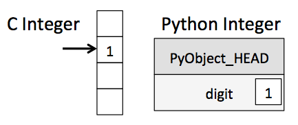
PyObject_HEAD是结构的一部分,包含引用计数,类型代码和之前提到的其他部分。注意这里的区别:C整数本质上是内存中位置的标签,其字节编码整数值。Python整数是指向内存中包含所有Python对象信息的位置的指针,包括包含整数值的字节。Python整数结构中的这些额外信息允许Python自由动态地编码。然而,Python类型中的所有这些附加信息都需要付出代价,这在组合了许多这些对象的结构中变得尤为明显。
Python列表不仅仅是一个列表现在让我们考虑当我们使用包含许多Python对象的Python数据结构时会发生什么。 Python中的标准可变多元素容器就是列表。我们可以创建一个整数列表,如下所示:
In [1]: L = list(range(10))
In [2]: L
Out[2]: [0, 1, 2, 3, 4, 5, 6, 7, 8, 9]
In [3]: type(L[0])
Out[3]: int
或者,类似地,字符串列表:
In [10]: L2 = [str(c) for c in L]
...: L2
Out[10]: ['0', '1', '2', '3', '4', '5', '6', '7', '8', '9']
In [11]: type(L2[0])
Out[11]: str
由于Python的动态类型,我们甚至可以创建异构列表:
In [12]: L3 = [True, "2", 3.0, 4]
...: [type(item) for item in L3]
Out[12]: [bool, str, float, int]
但是这种灵活性是有代价的:要允许这些灵活类型,列表中的每个项目都必须包含自己的类型信息,引用计数和其他信息 - 也就是说,每个项目都是完整的Python对象。在所有变量属于同一类型的特殊情况下,大部分信息都是多余的:将数据存储在固定类型数组中会更有效。动态类型列表和固定类型(NumPy样式)数组之间的区别如下图所示:
在实现级别,该数组实质上包含指向一个连续数据块的单个指针。另一方面,Python列表包含一个指向指针块的指针,每个指针指向一个完整的Python对象,就像我们之前看到的Python整数一样。同样,列表的优点是灵活性:因为每个列表元素是包含数据和类型信息的完整结构,所以列表可以填充任何所需类型的数据。固定类型NumPy样式的数组缺乏这种灵活性,但是对于存储和操作数据更有效。
Python提供了几种不同的选项,用于在高效的固定类型数据缓冲区中存储数据。内置的数组模块(自Python 3.3起可用)可用于创建统一类型的密集数组:
In [13]: import array
...: L = list(range(10))
...: A = array.array('i', L)
...: A
Out[13]: array('i', [0, 1, 2, 3, 4, 5, 6, 7, 8, 9])
这里'i'是一个类型代码,表示内容是整数。
然而,更有用的是NumPy包的ndarray对象。虽然Python的数组对象提供了基于数组的数据的高效存储,但NumPy在这些数据上增加了这种有效的操作。我们将在后面的章节中探讨这些操作;在这里,我们将演示创建NumPy数组的几种方法。
我们将从别名np下的标准NumPy导入开始:
import numpy as np
Python列表创建数组首先,我们可以使用np.array从Python列表创建数组:
# integer array:
In [14]: np.array([1, 4, 2, 5, 3])
Out[14]: array([1, 4, 2, 5, 3])
请记住,与Python列表不同,NumPy受限于所有包含相同类型的数组。如果类型不匹配,NumPy将尽可能向上转换(此处,整数向上转换为浮点数):
In [15]: np.array([3.14, 4, 2, 3])
Out[15]: array([3.14, 4. , 2. , 3. ])
如果我们想显式设置结果数组的数据类型,我们可以使用dtype关键字:
In [16]: np.array([1, 2, 3, 4], dtype='float32')
Out[16]: array([1., 2., 3., 4.], dtype=float32)
最后,与Python列表不同,NumPy数组可以明确地是多维的;这是使用列表列表初始化多维数组的一种方法:
# nested lists result in multi-dimensional arrays
In [17]: np.array([range(i, i + 3) for i in [2, 4, 6]])
Out[17]:
array([[2, 3, 4],
[4, 5, 6],
[6, 7, 8]])
内部列表被视为生成的二维数组的行。
特别是对于较大的阵列,使用NumPy内置的例程从头开始创建数组效率更高。以下是几个例子:
# 创建一个用零填充的长度为10的整数数组
In [18]: np.zeros(10, dtype=int)
Out[18]: array([0, 0, 0, 0, 0, 0, 0, 0, 0, 0])
# 创建一个填充了1的3x5的浮点数组
In [19]: np.ones((3, 5), dtype=float)
Out[19]:
array([[1., 1., 1., 1., 1.],
[1., 1., 1., 1., 1.],
[1., 1., 1., 1., 1.]])
# 创建一个填充3.14的3x5数组
In [20]: np.full((3, 5), 3.14)
Out[20]:
array([[3.14, 3.14, 3.14, 3.14, 3.14],
[3.14, 3.14, 3.14, 3.14, 3.14],
[3.14, 3.14, 3.14, 3.14, 3.14]])
# 创建一个填充线性序列的数组
# 从0开始,到20结束,步进2
# (这类似于内置range()函数)
In [21]: np.arange(0, 20, 2)
Out[21]: array([ 0, 2, 4, 6, 8, 10, 12, 14, 16, 18])
# 创建一个由0和1均匀分布的五个值的数组
In [22]: np.linspace(0, 1, 5)
Out[22]: array([0. , 0.25, 0.5 , 0.75, 1. ])
# 创建一个均匀分布的3x3数组
# 随机值介于0和1之间
In [23]: np.random.random((3, 3))
Out[23]:
array([[0.91398038, 0.24537985, 0.01826515],
[0.4294535 , 0.69789859, 0.55493684],
[0.12512603, 0.49085695, 0.66702286]])
# 创建3x3正态分布随机值数组
# 平均值为0,标准差为1
In [24]: np.random.normal(0, 1, (3, 3))
Out[24]:
array([[ 0.45408335, -1.90310333, -0.33322852],
[ 0.51879233, -0.03587706, 1.47226021],
[ 0.07377611, 0.35394745, -0.08673764]])
# 在区间[0,10]中创建3x3随机整数数组
In [25]: np.random.randint(0, 10, (3, 3))
Out[25]:
array([[0, 0, 1],
[4, 3, 1],
[0, 8, 5]])
# 创建3x3单位矩阵
In [26]: np.eye(3)
Out[26]:
array([[1., 0., 0.],
[0., 1., 0.],
[0., 0., 1.]])
# 创建一个包含三个整数的未初始化数组
# 值将是该内存位置已存在的任何值
In [27]: np.empty(3)
Out[27]: array([1., 1., 1.])
NumPy标准数据类型NumPy数组包含单一类型的值,因此详细了解这些类型及其限制非常重要。由于NumPy是用C构建的,因此C,Fortran和其他相关语言的用户会熟悉这些类型。
标准NumPy数据类型列在下表中。请注意,在构造数组时,可以使用字符串指定它们:
np.zeros(10, dtype='int16')
或者使用关联的NumPy对象:
np.zeros(10, dtype=np.int16)
| Data type | Description |
|---|---|
| bool_ | Boolean (True or False) stored as a byte |
| int_ | Default integer type (same as C long; normally either int64 or int32) |
| intc | Identical to C int (normally int32 or int64) |
| intp | Integer used for indexing (same as C ssize_t; normally either int32 or int64) |
| int8 | Byte (-128 to 127) |
| int16 | Integer (-32768 to 32767) |
| int32 | Integer (-2147483648 to 2147483647) |
| int64 | Integer (-9223372036854775808 to 9223372036854775807) |
| uint8 | Unsigned integer (0 to 255) |
| uint16 | Unsigned integer (0 to 65535) |
| uint32 | Unsigned integer (0 to 4294967295) |
| uint64 | Unsigned integer (0 to 18446744073709551615) |
| float_ | Shorthand for float64. |
| float16 | Half precision float: sign bit, 5 bits exponent, 10 bits mantissa |
| float32 | Single precision float: sign bit, 8 bits exponent, 23 bits mantissa |
| float64 | Double precision float: sign bit, 11 bits exponent, 52 bits mantissa |
| complex_ | Shorthand for complex128. |
| complex64 | Complex number, represented by two 32-bit floats |
| complex128 | Complex number, represented by two 64-bit floats |
更高级的类型规范是可能的,例如指定大或小的字节序数;有关更多信息,请参阅NumPy文档。NumPy还支持复合数据类型,这将在结构化数据中进行介绍:NumPy的结构化阵列。
本节介绍如何使用布尔掩码来检查和操作NumPy数组中的值。当您想要根据某些标准提取,修改,计数或以其他方式操纵数组中的值时,会出现屏蔽(Masking):例如,您可能希望计算所有大于某个值的值,或者可能删除超过某个阈值的所有异常值。在NumPy中,布尔掩码通常是完成这些类型任务的最有效方法。
想象一下,您有一系列数据表示某一城市一年中每天的降水量。例如,在这里,我们将使用Pandas(在第3章中详细介绍)加载2014年西雅图市的每日降雨量统计数据:
In [1]: import numpy as np
...: import pandas as pd
...:
...: # use pandas to extract rainfall inches as a NumPy array
...: rainfall = pd.read_csv('data/Seattle2014.csv')['PRCP'].values
...: inches = rainfall / 254.0 # 1/10mm -> inches
...: inches.shape
Out[1]: (365,)
该数组包含365个值,以2014年1月1日至12月31日的每日降雨量为单位。
作为第一个快速可视化,让我们看一下使用Matplotlib生成的雨天直方图(我们将在第4章中更全面地探讨这个工具):
In [2]: %matplotlib inline
...: import matplotlib.pyplot as plt
...: import seaborn; seaborn.set() # set plot styles
In [3]: plt.hist(inches, 40);
这个直方图让我们对数据的概况有了一个大概的了解:尽管它的声誉很高,但西雅图的绝大多数日子在2014年测得的降雨量几乎为零。但这并没有很好地传达我们希望看到的一些信息:例如,一年中有多少雨天?那些下雨天的平均降雨量是多少?有多少天有超过半英寸的降雨?
一种方法是手动回答这些问题:循环数据,每当我们看到某个所需范围内的值时递增计数器。由于本章中讨论的原因,从编写代码的时间和计算结果的时间的角度来看,这种方法效率非常低。我们在NumPy Arrays的计算:通用函数中看到,可以使用NumPy的ufunc代替循环来对数组进行快速的逐元素算术运算;以同样的方式,我们可以使用其他ufunc对数组进行逐元素比较,然后我们可以操纵结果来回答我们的问题。我们现在暂时搁置数据,来讨论NumPy中的一些常用工具,以使用屏蔽来快速回答这些类型的问题。
ufuncs在NumPy数组计算:通用函数里,我们介绍了ufuncs,特别关注算术运算符。我们看到在数组上使用+, - ,*,/和其他运算会导致逐元素操作。NumPy还实现了例如<(小于)和>(大于)的逐元素方的比较运算ufunc。这些比较运算符的结果始终是具有布尔数据类型的数组。所有六种标准比较操作都可用:
In [5]: x = np.array([1, 2, 3, 4, 5])
In [6]: x < 3 # less than
Out[6]: array([ True, True, False, False, False])
In [7]: x > 3 # greater than
Out[7]: array([False, False, False, True, True])
In [8]: x <= 3 # less than or equal
Out[8]: array([ True, True, True, False, False])
In [9]: x >= 3 # greater than or equal
Out[9]: array([False, False, True, True, True])
In [10]: x != 3 # not equal
Out[10]: array([ True, True, False, True, True])
In [11]: x == 3 # equal
Out[11]: array([False, False, True, False, False])
也可以对两个数组进行逐元素比较,并包含复合表达式:
In [14]: (2 * x) == (x ** 2)
Out[14]: array([False, True, False, False, False])
与算术运算符的情况一样,比较运算符在NumPy中实现为ufunc;例如,当你写x <3时,内部NumPy使用np.less(x,3)。此处显示了比较运算符及其等效ufunc的摘要:
| Operator | Equivalent ufunc | Operator | Equivalent ufunc |
|---|---|---|---|
| == | np.equal | != | np.not_equal |
| < | np.less | <= | np.less_equal |
|np.greater|>=|np.greater_equal
就像算术ufuncs的情况一样,这些将适用于任何大小和形状的数组。这是一个二维的例子:
In [15]: rng = np.random.RandomState(0)
...: x = rng.randint(10, size=(3, 4))
...: x
Out[15]:
array([[5, 0, 3, 3],
[7, 9, 3, 5],
[2, 4, 7, 6]])
In [16]: x < 6
Out[16]:
array([[ True, True, True, True],
[False, False, True, True],
[ True, True, False, False]])
在每种情况下,结果都是一个布尔数组,NumPy提供了许多简单的模式来处理这些布尔结果。
给定一个布尔数组,您可以执行许多有用的操作。我们将使用x,我们之前创建的二维数组。
In [17]: print(x)
[[5 0 3 3]
[7 9 3 5]
[2 4 7 6]]
要计算布尔数组中True条目的数量,np.count_nonzero非常有用:
In [18]: # how many values less than 6?
...: np.count_nonzero(x < 6)
Out[18]: 8
我们看到有8个小于6的数组条目。获取此信息的另一种方法是使用np.sum;在这种情况下,False被解释为0,而True被解释为1:
In [19]: np.sum(x < 6)
Out[19]: 8
sum()的好处是与其他NumPy聚合函数一样,这个求和也可以沿着行或列完成:
In [20]: np.sum(x < 6, axis=1)
Out[20]: array([4, 2, 2])
这就是计算矩阵中每行小于6的值的数量。
如果我们有兴趣快速检查是否有任何或所有值都是真的,我们可以使用(你猜对了)np.any或np.all:
In [21]: # are there any values greater than 8?
...: np.any(x > 8)
Out[21]: True
In [22]: # are there any values less than zero?
...: np.any(x < 0)
Out[22]: False
In [23]: # are all values less than 10?
...: np.all(x < 10)
Out[23]: True
In [24]: # are all values equal to 6?
...: np.all(x == 6)
Out[24]: False
np.all和np.any也可以沿特定轴使用。例如:
In [25]: # are all values in each row less than 8?
...: np.all(x < 8, axis=1)
Out[25]: array([ True, False, True])
里第一行和第三行中的所有元素都小于8,而第二行则不是这种情况。
最后,一个快速警告:如Aggregations:Min,Max和Everything In Between中提到的,Python内置了sum(),any()和all()函数。它们的语法与NumPy版本不同,特别是在多维数组上使用时会失败或产生意外结果。确保您对这些示例使用np.sum(),np.any()和np.all()!
我们已经看到了我们如何计算,比如雨天小于4英寸的所有日子,或雨水大于2英寸的所有日子。但是,如果我们想了解雨量小于4英寸且大于1英寸的所有日子呢?
这是通过Python的按位逻辑运算符&,|,^来实现的。与标准算术运算符一样,NumPy将这些作为ufuncs重载,这些ufuncs在(通常是布尔)数组上按元素方式工作。
例如,我们可以解决这种复合问题如下:
In [26]: np.sum((inches > 0.5) & (inches < 1))
Out[26]: 29
所以我们看到有29天的降雨量在0.5到1.0英寸之间。
请注意,此处的括号很重要 - 由于运算符优先级规则,删除了括号,此表达式将按如下方式计算,这会导致错误:
inches > (0.5 & inches) < 1
使用A AND B和NOT(不是A或非B)的等价(如果你已经学过入门逻辑课程,你可能还记得),我们可以用不同的方式计算相同的结果:
In [27]: np.sum(~( (inches <= 0.5) | (inches >= 1) ))
Out[27]: 29
在数组上组合比较运算符和布尔运算符可以实现广泛的高效逻辑运算。
下表总结了按位布尔运算符及其等效的ufunc:
| Operator | Equivalent ufunc | Operator | Equivalent ufunc |
|---|---|---|---|
| & | np.bitwise_and | | | np.bitwise_or |
| ^ | np.bitwise_xor | ~ | np.bitwise_not |
使用这些工具,我们可能会开始回答有关天气数据的问题类型。以下是我们在将masking与聚合相结合时可以计算的一些结果示例:
In [28]: print("Number days without rain: ", np.sum(inches == 0))
...: print("Number days with rain: ", np.sum(inches != 0))
...: print("Days with more than 0.5 inches:", np.sum(inches > 0.5))
...: print("Rainy days with < 0.2 inches :", np.sum((inches > 0) &
...: (inches < 0.2)))
Number days without rain: 215
Number days with rain: 150
Days with more than 0.5 inches: 37
Rainy days with < 0.2 inches : 75
在上一节中,我们研究了直接在布尔数组上计算的聚合。更强大的模式是使用布尔数组作为掩码,以选择数据本身的特定子集。从之前返回我们的x数组,假设我们想要一个数组中所有值小于5的数组:
In [29]: x
Out[29]:
array([[5, 0, 3, 3],
[7, 9, 3, 5],
[2, 4, 7, 6]])
我们可以很容易地获得这种情况的布尔数组,正如我们已经看到的:
In [30]: x < 5
Out[30]:
array([[False, True, True, True],
[False, False, True, False],
[ True, True, False, False]])
现在要从数组中选择这些值,我们可以简单地索引这个布尔数组;这被称为掩蔽操作:
In [31]: x[x < 5]
Out[31]: array([0, 3, 3, 3, 2, 4])
返回的是一维数组,其中包含满足此条件的所有值;换句话说,掩码数组为True的位置中的所有值。
然后,我们可以随意对这些价值进行操作。例如,我们可以计算西雅图雨量数据的一些相关统计数据:
In [32]: # construct a mask of all rainy days
...: rainy = (inches > 0)
...:
...: # construct a mask of all summer days (June 21st is the 172nd day)
...: days = np.arange(365)
...: summer = (days > 172) & (days < 262)
...:
...: print("Median precip on rainy days in 2014 (inches): ",
...: np.median(inches[rainy]))
...: print("Median precip on summer days in 2014 (inches): ",
...: np.median(inches[summer]))
...: print("Maximum precip on summer days in 2014 (inches): ",
...: np.max(inches[summer]))
...: print("Median precip on non-summer rainy days (inches):",
...: np.median(inches[rainy & ~summer]))
Median precip on rainy days in 2014 (inches): 0.19488188976377951
Median precip on summer days in 2014 (inches): 0.0
Maximum precip on summer days in 2014 (inches): 0.8503937007874016
Median precip on non-summer rainy days (inches): 0.20078740157480315
通过组合布尔运算,掩码操作和聚合,我们可以非常快速地为我们的数据集回答这些问题。
and/or与运算符&/|一个常见的混淆点是关键字and和or,以及另一方面运算符&和|之间的差异。你什么时候使用其中一个而不是另一个?
区别在于:and和or衡量整个对象的真实性或虚假性,而&和|指向对象中的每一位。
In [33]: bool(42), bool(0)
Out[33]: (True, False)
In [34]: bool(42 and 0)
Out[34]: False
In [35]: bool(42 or 0)
Out[35]: True
当你在整数上使用&和|时,对元素的位进行表达式操作,将and或or应用于构成数字的各个位:
In [36]: bin(42)
Out[36]: '0b101010'
In [37]: bin(59)
Out[37]: '0b111011'
In [38]: bin(42 & 59)
Out[38]: '0b101010'
In [39]: bin(42 | 59)
Out[39]: '0b111011'
请注意,比较二进制表示的相应位以产生结果。
当你在NumPy中有一个布尔值数组时,这可以被认为是一串位,其中1 = True,0 = False,&和|的结果与上述类似的操作:
In [40]: A = np.array([1, 0, 1, 0, 1, 0], dtype=bool)
...: B = np.array([1, 1, 1, 0, 1, 1], dtype=bool)
...: A | B
Out[40]: array([ True, True, True, False, True, True])
使用或在这些数组上将尝试评估整个数组对象的真实性或虚假性,这不是一个明确定义的值:
In [41]: A or B
---------------------------------------------------------------------------
ValueError Traceback (most recent call last)
<ipython-input-41-ea2c97d9d9ee> in <module>
----> 1 A or B
ValueError: The truth value of an array with more than one element is ambiguous. Use a.any() or a.all()
类似地,在给定数组上执行布尔表达式时,应使用|或者而不是or或者and:
In [42]: x = np.arange(10)
...: (x > 4) & (x < 8)
Out[42]:
array([False, False, False, False, False, True, True, True, False,
False])
试图评估整个数组的真实性或错误性会产生我们之前看到的相同的ValueError:
In [43]: (x > 4) and (x < 8)
---------------------------------------------------------------------------
ValueError Traceback (most recent call last)
<ipython-input-43-eecf1fdd5fb4> in <module>
----> 1 (x > 4) and (x < 8)
ValueError: The truth value of an array with more than one element is ambiguous. Use a.any() or a.all()
所以请记住:and和or对整个对象执行单个布尔评估,而&和|对对象的内容(单个位或字节)执行多个布尔评估。对于布尔NumPy数组,后者几乎总是所需的操作。
注:masking翻译软件译作“掩码”感觉挺怪的,但是行业里又不知道该如何翻译,只能留待以后更正。
| 快捷键 | 动作 |
|---|---|
Ctrl-a |
将光标移动到行的开头 |
Ctrl-e |
将光标移动到行的结尾 |
Ctrl-b /左箭头 |
将光标移回(左)一个字符 |
Ctrl-f /右箭头 |
将光标向前(右)移动一个字符 |
退格键删除前(左)一个字符
| 快捷键 | 动作 |
|---|---|
Ctrl-d |
删除下一个(右边)字符 |
Ctrl-k |
剪切从光标切换到行尾的文本 |
Ctrl-u |
剪切从光标切换到行首的文本 |
Ctrl-y |
粘贴上次剪切的文本 |
Ctrl-t |
转换光标前两个字符 |
也许这里讨论的最有影响力的快捷方式是IPython为导航命令历史记录提供的快捷方式。此命令历史记录超出了当前的IPython会话:您的整个命令历史记录存储在IPython配置文件目录中的SQLite数据库中。
访问这些的最直接的方法是使用向上和向下箭头键来逐步浏览历史记录,但也存在其他选项:
| 快捷键 | 动作 |
|---|---|
Ctrl-p /身上箭头 |
访问历史记录中的上一个命令 |
Ctrl-n/向下箭头 |
访问历史记录中的下一个命令 |
Ctrl-r |
反向搜索命令历史记录 |
| 如果您在此提示符下开始键入字符,IPython将自动填充与这些字符匹配的最新命令(如果有): |
In [1]:
(reverse-i-search)`sqa': square??
在任何时候,您都可以添加更多字符来优化搜索,或再次按Ctrl-r进一步搜索与查询匹配的其他命令。如果您按照上一节中的说明进行操作,则再次按Ctrl-r可以:
In [1]:
(reverse-i-search)`sqa': def square(a):
"""Return the square of a"""
return a ** 2
找到要查找的命令后,按Return键,搜索结束。然后我们可以使用检索到的命令,并随身携带我们的会话:
In [1]: def square(a):
"""Return the square of a"""
return a ** 2
In [2]: square(2)
Out[2]: 4
请注意,Ctrl-p / Ctrl-n或向上/向下箭头键也可用于搜索历史记录,但只能通过匹配行开头的字符。也就是说,如果您键入def然后按Ctrl-p,它将在历史记录中找到以字符def开头的最新命令(如果有)。
| 快捷键 | 动作 |
|---|---|
Ctrl-l |
清除终端屏幕 |
Ctrl-c |
中断当前的Python命令 |
Ctrl-d |
退出IPython会话 |
Visual Studio Code安装插件主要有两种方式
按F1,然后输入:extensions: Install Extensions,按回车即可。

CTRL + P 然后输入 ext install,按回车即可。

在左侧搜索栏输入Markdown Preview Enhanced,安装即可。

爬取某网站上的内容时,获取到html内容成功
# coding: utf-8
import requests
from lxml import etree
start_url = 'http://wap.ynpxrz.com/n1413623c2181.aspx'
r = requests.get(start_url)
e = etree.fromstring(r.text)
# print(r.text)
print(e)
但是使用lxml解释的时候,却报错了:
Traceback (most recent call last):
File "E:/DEV/projects/spider/demo.py", line 10, in <module>
e = etree.fromstring(r.text)
File "src\lxml\etree.pyx", line 3222, in lxml.etree.fromstring
File "src\lxml\parser.pxi", line 1877, in lxml.etree._parseMemoryDocument
File "src\lxml\parser.pxi", line 1758, in lxml.etree._parseDoc
File "src\lxml\parser.pxi", line 1068, in lxml.etree._BaseParser._parseUnicodeDoc
File "src\lxml\parser.pxi", line 601, in lxml.etree._ParserContext._handleParseResultDoc
File "src\lxml\parser.pxi", line 711, in lxml.etree._handleParseResult
File "src\lxml\parser.pxi", line 640, in lxml.etree._raiseParseError
File "<string>", line 19
lxml.etree.XMLSyntaxError: Opening and ending tag mismatch: link line 16 and head, line 19, column 8
看到XMLSyntaxError,我猜大概是解释器使用不当造成的。
给fromstring方法指定parse参数:
e = etree.fromstring(r.text, parser=etree.HTMLParser())
问题解决了。
A declarative, efficient, and flexible JavaScript library for building user interfaces.
🖖 Vue.js is a progressive, incrementally-adoptable JavaScript framework for building UI on the web.
TypeScript is a superset of JavaScript that compiles to clean JavaScript output.
An Open Source Machine Learning Framework for Everyone
The Web framework for perfectionists with deadlines.
A PHP framework for web artisans
Bring data to life with SVG, Canvas and HTML. 📊📈🎉
JavaScript (JS) is a lightweight interpreted programming language with first-class functions.
Some thing interesting about web. New door for the world.
A server is a program made to process requests and deliver data to clients.
Machine learning is a way of modeling and interpreting data that allows a piece of software to respond intelligently.
Some thing interesting about visualization, use data art
Some thing interesting about game, make everyone happy.
We are working to build community through open source technology. NB: members must have two-factor auth.
Open source projects and samples from Microsoft.
Google ❤️ Open Source for everyone.
Alibaba Open Source for everyone
Data-Driven Documents codes.
China tencent open source team.