InfoGAN, an information-theoretic extension to the GAN that is able to learn disentangled representations in a completely unsupervised manner. (Related to #33)
Problem: Input noise vector z has no restrictions on the manner in which the generator may use this noise. As a result, it is possible that the noise will be used by the generator in a highly entangled way, causing the individual dimensions of z to not correspond to semantic features of the data.
InfoGAN
Decompose the input noise vector z into 2 parts:
Incompressible noise z (interpret as an uncertainty of dataset that cannot be encoded to meaningful factors of variation)
Disentangled latent code c = {c_1, c_2, ..., c_L} (Encode factors of variation of dataset)
Note both vectors are learned in an unsupervised manner.
Problem: The generator may ignore the latent code: P_G(x|c) = P_G(x).
Apply regularization by maximizing mutual information: I(c; G(z,c)).
Mutual information I(X;Y):
Measures the “amount of information” learned from knowledge of random variable Y about the other random variable X.
I(X;Y) = H(X) − H(X|Y) = H(Y) − H(Y|X), where H(.) is entropy.
I(X;Y) is the reduction of uncertainty in X when Y is observed. If X and Y are independent, then I(X;Y) = 0, because knowing one variable reveals nothing about the other.
Given any x ∼ P_G(x), we want P_G(c|x) to have a small entropy. In other words, the information in the latent code c should not be lost in the generation process (Address the above problem).
This paper focuses on domain adaption issues in RL settings where an agent trained on a particular input distribution with a specified reward structure (source domain) is modified but the reward structure remains largely intact (target domain). The target domain can be unknown.
This paper aims to develop an agent that can learn a robust policy using observations and rewards obtained exclusively within the source domain. Here, a policy is considered as robust if it generalizes with minimal drop in performance to the target domain without extra fine-tuning.
This paper tackles the domain adaption problem by learning a disentangled/factorized representation of the world. Examples of such factors of variation in the world are object properties like color, scale, or position; other examples correspond to general environmental factors, such as geometry and lighting.
The purposed system, DARLA, relies on learning a latent state representation that is shared between the source and target domains, by learning a disentangled representation of the environment’s generative factors. Crucially, DARLA does not require target domain data to form its representations.
Framework
Formalized problem setting
The source domain D_{S} ≡ (S_{S}, A_{S}, T_{S}, R_{S}).
The target domain D_{T} ≡ (S_{T}, A_{T}, T_{T}, R_{T}).
Where S: State; A: Action; T: Transition function; R: Reward.
For example. Robot arm in simulated environment and real world: S: Raw pixels; A: Robot's action; T: Physics of the world; R: The performance on the task.
DARLA
Three stages pipeline:
Learning to see (the main contribution):
Use a random policy to interact with environment to collect observations (require sufficient variability of factors and their conjunctions).
However, the shortcomings of reconstructing in pixel space are known and have been addressed in reconstruction in feature space given by another neural network. (e.g., GAN or pretrained AlexNet)
In practice, this paper found that using a denoising autoencoder (DAE) for β-VAE works best.
In detail, they follow the masking noise of [1] with the aim for the DAE to learn a semantic representation of the input frames.
Problem: The DAE might also suffer from domain adapation problem. If the semantic representation learned by DAE doesn't transfer well from source to target domain, the β-VAE, which depends on DAE, will also suffer.
After pretraining DAE, train β-VAE for reconstruction in DAE's feature space using L2 distance. DAE remains frozen.
Learning to act: The agent is tasked with learning the source policy via a standard RL algorithms (DQN, A3C and Episodic Control). The parameters of the encoder (which encodes raw pixels to internal state for the decoder to predict actions) of agent will not be updated. They also compared with UNREAL.
Transfer: Since the encoder already learns the disentangled representation of the world of source domain, such a policy would then generalize well to the target domain out-of-the-box. In this stage, we simply evaluate the agent in target domain without retraining.
Object detection typically assumes that training and test data are drawn from an identical distribution, which, however, does not always hold in practice. Such a distribution mismatch will lead to a significant performance drop.
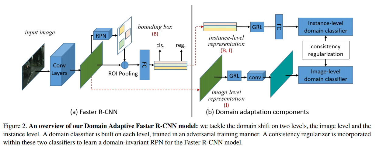
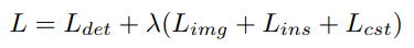
Two domain shifts are tackled: (1) image level adaptation (2) instance level adaptation.
Contributions
We provide a theoretical analysis of the domain shift problem for cross-domain object detection from a probabilistic perspective.
We design two domain adaptation components to alleviate the domain discrepancy at the image and instance levels, resp.
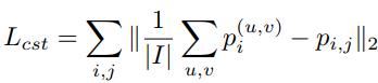
We further propose a consistency regularization to encourage the RPN to be domain-invariant.
We integrate the proposed components into the Faster R-CNN model, and the resulting system can be trained in an end-to-end manner.
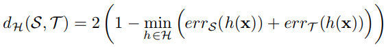
H-divergence Definition
The H-divergence [1] is designed to measure the divergence between two sets of samples with different distributions.
H-divergence definition:
h(.) is a feature-level domain classifier, if the error is high for the best domain classifier, the two domains are hard to distinguish, so they are close to each other, and vice versa.
To align source and target domains, minimize the domain distance, which maximize the H-divergence.
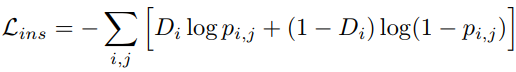
Given the same image region containing an object, its category labels should be the same regardless of which domain it comes from.
Joint adaptation:
Consider P(B, I) = P(B|I) x P(I)
P(B|I) is assumed to be the same under covariate shift assumption.
Thus if P_{S} (I) = P_{T} (I), we have P_{S} (B, I) = P_{T} (B, I)
In other words, if the distributions of the image-level representations are identical for two domains, the distributions of the instance-level representations are also identical.
Yet, it is generally non-trivial to perfectly estimate the conditional distribution P(B|I), since:
In practice it may be hard to perfectly align the marginal distributions P(I), which means the input for estimating P(B|I) is somehow biased.
The bounding box annotation is only available for source domain training data, therefore P(B|I) is learned using the source domain data only, which is easily biased toward the source domain.
Method
We propose to perform domain distribution alignment on both the image and instance levels, and to apply a consistency regularization to alleviate the bias in estimating P(B|I).
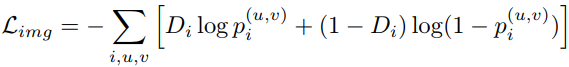
To align the source and target domain, train a domain classifier, thus we have 2 domain classifier:
Notation: D denotes domain label.
Image-level domain classifier: P(D|I)
Instance-level domain classifier: P(D|B, I)
By Bayes’ theorem: P(D|B, I) P(B|I) = P(B|D, I) P(D|I).
By enforcing the consistency between two domain classifiers, i.e., P(D|B, I) = P(D|I), we could learn P(B|D, I) to approach P(B|I).
Region Proposal Networks: A FCN (fully convolution network) that proposes regions. (Serve as the "attention" for Fast-RCNN)
Fast R-CNN [1]: A classifier that uses proposed regions.
Region Proposal Networks (RPN)
Input: An image of any size.
Output: A set of rectangular object proposals, each with an objectness score.
Slide a small network over the last conv. feature map.
Input: n x n spatial window of conv. feature map. (n = 3 in this paper)
Each spatial window is projected to feature vector (512-d for VGG-16), then fed into two sibling FCs, a box-regression layer (reg) and a box classification layer (cls).
This architecture is naturally implemented with an n × n conv. layer followed by two sibling 1 × 1 conv. layers (for reg and cls, respectively).
For each spatial (sliding) window, multiple regions proposals (boxes) are predicted simultaneously, where the number of maximum possible proposals for each location is denoted as k.
The reg layer outputs 4k (coordinates of k boxes)
The cls layer outputs 2k scores of being a object or not for k boxes.
The k proposals are parameterized relative to k reference boxes, which we call anchors.
Anchor: An anchor is centered at the sliding window in question, and is associated with a scale and aspect ratio. (This paper uses 3 scales and 3 aspect ratios, yielding k = 9 anchors at each sliding position. For conv. feature map of a size W × H (typically ∼2,400), there are W x H x k anchors in total.
RPN is translation-invariant. (Guarantee that the same proposal is generated if an object is translated).
(4 + 2) x 9-d conv. output layer in the case of k = 9 anchors.
A pyramid of anchors: Our method classifies and regresses bounding boxes with reference to anchor boxes of multiple scales and aspect ratios.
It only relies on images and feature maps of a single scale, and uses filters (sliding windows on the feature map) of a single size.
The design of multi-scale anchors is a key component for sharing features without extra cost for addressing scales.
Loss function:
Binary label (being an object or not) for each anchor.
Positive label:
The anchor/anchors with the highest Intersection-over-Union (IoU) overlap with a ground-truth box.
An anchor that has an IoU overlap higher than 0.7 with any ground-truth box.
Note that a single ground-truth box may assign positive labels to multiple anchors.
Negative label: The anchor's IoU ratio is lower than 0.3 for all ground-truth boxes.
Anchors that are neither positive nor negative do not contribute to the training objective.
Minimize the multi-task loss in Fast R-CNN:
i: An index of an anchor in a mini-batch; p_{i}: Prob. of being an object; t_{i}: A vector representing the 4 parameterized coordinates of the predicted bounding box; *t_{i}**: Ground-truth bounding boxes associated with a positive anchor.
L_{cls}: log-loss; L_{reg}: smoothed L1 loss.
Parameterizations of the 4 coordinates:
x, y, w, and h denote the box’s center coordinates and its width and height.
Variables x, x_{a}*, and x are for the predicted box, anchor box, and ground-truth box respectively (likewise for y, w, h).
Can be thought of as bounding-box regression from an anchor box to a nearby ground-truth box.
Bounding-box regression: The features used for regression are of the same spatial size (3 × 3) on the feature maps. To account for varying sizes, a set of k bounding-box regressors are learned. Each regressor is responsible for one scale and one aspect ratio, and the k regressors do not share weights. As such, it is still possible to predict boxes of various sizes even though the features are of a fixed size/scale, thanks to the design of anchors.
Training:
Follow the "image-centric" sampling strategy [1].
It is possible to optimize for the loss functions for all anchors, but this will bias toward negative samples as they are dominated.
Randomly sample 256 anchors in an image where positive:negative = 1:1. Pad the mini-batch with negative ones if there're fewer than 128 positive sample anchors.
Adopt 4-Step Alternating Training
Initialized with ImageNet-pretrained model and fine-tuned end-to-end for the region proposal task.
Train a separate detection network (also initialized with ImageNet-pretrained model) by Fast R-CNN using the proposals generated by the step-1 RPN.
At this point the two networks do not share conv. layers.
Use the detector network to initialize RPN training, but we fix the shared conv. layers and only fine-tune the layers unique to RPN.
Finally, keeping the shared conv. layers fixed, we fine-tune the unique layers of Fast R-CNN.
Implementation and hyperparameter details are provided in the paper.
In this note, I'll continue recording several findings whatever I think it's important or useful. I'll be focusing on the theoretical and heuristic parts in several GANs papers. This thread will be actively updated whenever I read a GANs paper! 😊
Notations:
p_{data}: Probability density/mass function of real data.
p_{g}/{d}: Probability density/mass function of generator/discriminator.
For G fixed, the optimal D is: D*{G} (x) = p{data}(x) / (p_{data}(x) + p_{g}(x)).
Global optimality: GANs has a global optimum for p_{g} = p_{data} (i.e., the generator perfectly replicating the real data distribution).
Essentially, the loss function of GAN quantifies the similarity between the p_{g} and p_{data} by JS divergence (symmetric) when the discriminator is optimal.
Convergence: If G and D have enough capacity, and at each step of training, the discriminator is allowed to reach its optimum, given G, and p_{g} is updated so as to improve the criterion then p_{g} converges to p_{data}.
G must not be trained too much without updating D, in order to avoid mode collapse in G.
Note: The discussion is under the scope of vanilla GANs.
Training GANs requires finding the Nash equilibrium of a game, which is a more difficult problem than optimizing an objective function.
Simply flipping the sign on the discriminator's objective function for the generator (i.e., maximizing the cross-entropy loss of the discriminator) could make the generator's gradient be vanished when the discriminator successfully rejects generator samples with high confidence.
MLE (maximum likelihood estimation) is equivalent to minimizing KL divergence KL(p_{data} || p_{g}).
VAE (variational autoencoder) v.s. GAN: VAE maximizes MLE but GANs aims to generate realistic samples instead of maximizing MLE.
GANs minimizes JS divergence which is similar to minimizing reverse KL divergence (i.e. KL(p_{g} || p_{data}). (KL divergence is not symmetric).
GANs do not use MLE, but it can be do so by modifying the generator's objective function, under the assumption that the discriminator is optimal. GANs still generate realistic samples even using MLE. (See the paper "On Distinguishability Criteria for Estimating Generative Models" by Goodfellow. ICLR 2015. Also see the video at 55:00). Thus, the choice of the divergence (KL v.s. reverse KL) cannot explain why GANs can generate realistic samples.
Maybe it is the approximation strategy of using supervised learning to estimate the density ratio that leads to the generated samples very realistic. (See the video at 59:15)
GANs often choose to generate from very few modes; fewer than the limitation imposed by the model capacity. The reverse KL prefers to generate from as many modes of the data distribution as the model is able to; it does not prefer fewer modes in general. This suggests that the mode collapse is driven by a factor other than the choice of divergence.
Mode collapse is believed not be caused by minimizing the reverse KL, since minimizing the forward KL still happens mode collapse. The deficiency design of minimax game could be a reason causing mode collapse. See the paper "Unrolled Generative Adversarial Networks" that successfully generate different modes of data.
Model architectures that cannot capture global structure will cause generated images with wrong global structure.
β-VAE is a state of the art model for unsupervised visual disentangled representation learning.
β-VAE adds an extra hyperparameter β to the VAE objective, which constricts the effective encoding capacity of the latent bottleneck and encourages the latent representation to be more factorized.
The disentangled representations learned by β-VAE have been shown to be important for learning a hierarchy of abstract visual concepts conducive of imagination (SCAN, Higgins et al.) and for improving transfer performance of reinforcement learning policies, including simulation to reality transfer in robotics (DARLA. Higgins et al.)
Motivation
It is currently unknown what causes the factorized representations learnt by β-VAE to be axis aligned with the human intuition of the data generative factors compared to the standard VAE.
Furthermore, β-VAE has other limitations, such as worse reconstruction fidelity compared to the standard VAE. This is caused by a trade-off introduced by the modified training objective that punishes reconstruction quality in order to encourage disentanglement within the latent representations.
This paper attempts to shed light on the question of why β-VAE disentangles, and to use the new insights to suggest practical improvements to the β-VAE framework to overcome the reconstruction-disentanglement trade-off.
Understanding disentangling in β-VAE
From information bottleneck principle (Tishby et al. 1999) perspective, the β-VAE training objective encourages the latent distribution q(z|x) to efficiently transmit information about the data points x by jointly minimizing the β-weighted KL term and maximizing the data log likelihood.
A strong pressure for overlapping posteriors encourages β-VAE to find a representation space preserving as much as possible the locality of points on the data manifold.
Hypothesis: β-VAE finds latent components which make different contributions to the log-likelihood term of the objective function. These latent components tend to correspond to features in the data that are intuitively qualitatively different, and therefore may align with the generative factors in the data.
For example, consider optimizing the β-VAE objective under an almost complete information bottleneck constraint (i.e. β >> 1). The optimal thing to do in this scenario is to only encode information about the data points which can yield the most significant improvement in data log-likelihood (i.e. Eq(z|x)[log p(x|z)]).
Intuition of Improvement (The most important part)
For example, in the dSprites dataset (consisting of white 2D sprites varying in position, rotation, scale and shape rendered onto a black background) the model might only encode the sprite position under such a constraint. Intuitively, when optimizing a pixel-wise decoder log likelihood, information about position will result in the most gains compared to information about any of the other factors of variation in the data, since the likelihood will vanish if reconstructed position is off by just a few pixels.
Continuing this intuitive picture, we can imagine that if the capacity of the information bottleneck were gradually increased, the model would continue to utilize those extra bits for an increasingly precise encoding of position, until some point of diminishing returns is reached for position information, where a larger improvement can be obtained by encoding and reconstructing another factor of variation in the dataset, such as sprite scale.
They further test this intuition by training a model to generate dSprites conditioned on ground truth factors, with a controllable information bottleneck. Each factor is independently scaled by a learnable parameter and are subject to independently scaled additive noise (also learned), similar to the reparameterized latent distribution in β-VAE. Throughout the training, the capacity of information bottleneck increases linearly. The experiment shows that the early capacity is allocated to positional latents only (x and y), followed by a scale latent, then shape and orientation latents.
Original Paper: http://aclweb.org/anthology/P18-1097 (present a detailed comparison and analysis for different fluency boost learning and inference methods, which isn't summarized here.)
Authors: Shamil Chollampatt and Hwee Tou Ng1
Organization: National University of Singapore
Release Date: 2018 on Arxiv
Link: https://arxiv.org/pdf/1801.08831.pdf