-
转载请注明作者和出处: https://zhuanlan.zhihu.com/p/40447996
-
Github代码获取:https://github.com/jiguang123/Credit-Loans-of-Data-Analysis
-
Python版本: Python3.6
-
运行环境: Win10 + Anaconda + jupyter Notebook + Sublime text3
- 采用了Lending Club 信用贷款违约数据是美国网络贷款平台 LendingClub 在2007-2015年间的信用贷款情况数据,主要包括贷款状态和还款信息。附加属性包括:信用评分、地址、邮编、所在州等,累计75个属性(列),890000笔 贷款(行)。
- 贷款违约预测模型,使用了Numpy,Pandas,Sklearn科学计算包完成数据清洗,构建特征工程,以及完成预约模型的训练,数据可视化采用了Matplotlib及Seaborn等可视化包。
接下来,我们将利用给定的借贷数据,做一次较为完整的数据分析,进一步熟悉数据分析的流程。我们将分三个阶段来完成,分别是
-
数据的初步分析和整理
-
数据的探索性分析及可视化
-
借贷违约预测(LogisticRegression)
#导入相关库
import numpy as np
import pandas as pd

%matplotlib inline
import matplotlib.pyplot as plt
plt.style.use('ggplot')  #风格设置近似R这种的ggplot库

import seaborn as sns
sns.set_style('whitegrid')
导入LendingClub贷款数据
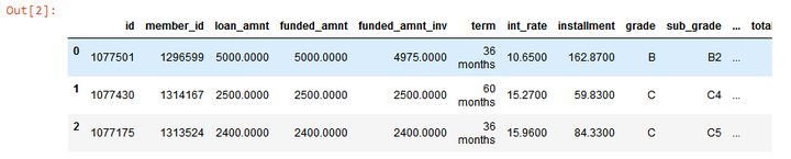
#导入数据及预览前三行
data=pd.read_csv("./dataset/loan.csv")
data.head(3)
本人电脑配置有限,为了加快计算速度,仅仅选择2015年度的贷款数据
#选择2015年度的贷款数据
data_15=data[(data.issue_d=='Jan-2015')\
            |(data.issue_d=='Feb-2015')\
            |(data.issue_d=='Mar-2015')\
            |(data.issue_d=='Apr-2015')\
            |(data.issue_d=='Apr-2015')\
            |(data.issue_d=='Apr-2015')\
            |(data.issue_d=='May-2015')\
            |(data.issue_d=='Jun-2015')\
            |(data.issue_d=='Jul-2015')\
            |(data.issue_d=='Aug-2015')\
            |(data.issue_d=='Sep-2015')\
            |(data.issue_d=='Oct-2015')\
            |(data.issue_d=='Nov-2015')\
            |(data.issue_d=='Dec-2015')\
            ]
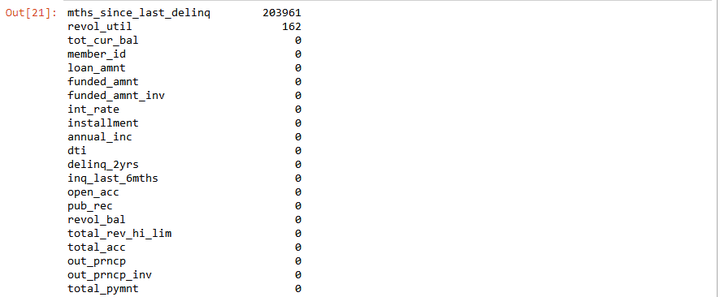
统计2015年度数据每列的缺失值情况。
#统计每列的缺失值情况
check_null = data_15.isnull().sum(axis=0).sort_values(ascending=False)/float(len(data)) #查看缺失值比例
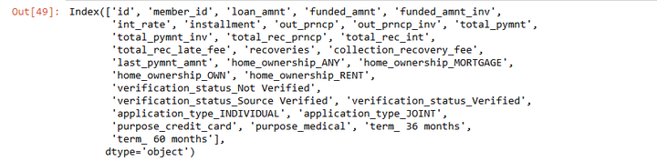
print(check_null[check_null > 0.2]) # 查看缺失比例大于20%的属性。
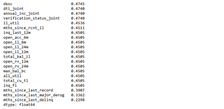
从上图中可以看出,数据集中有很多列都有缺失值,所以我们要判断此列的数据对预测结果是否有影响,如果没有影响,可以将此列删除,本文中我们将缺失值超过40%的列删除。
#删除缺失值超过40%的列
thresh_count = len(data_15)*0.4 # 设定阀值
data_15 = data_15.dropna(thresh=thresh_count, axis=1 ) #若某一列数据缺失的数量超过阀值就会被删除
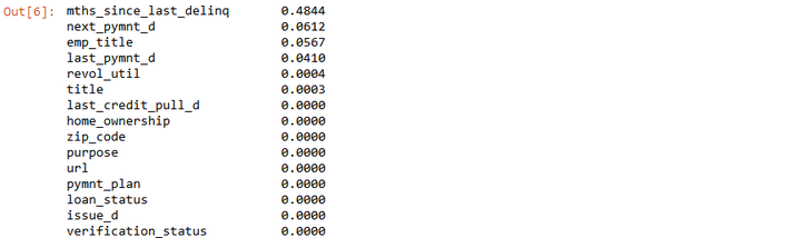
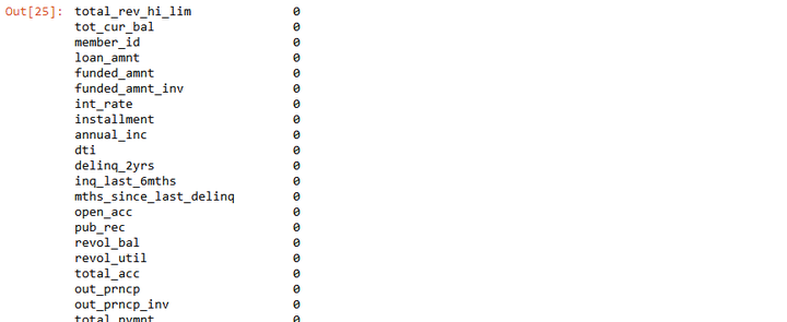
再次检查缺失值的情况,只有6列的数据还有缺失值。
#按缺失值比例从大到小排列
data_15.isnull().sum(axis=0).sort_values(ascending=False)/float(len(data_15))
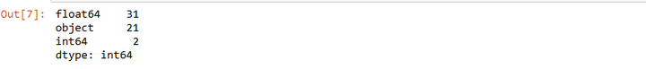
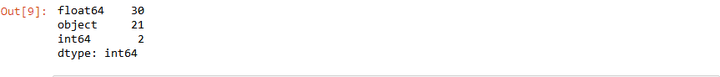
查看数据类型的大概分布情况
data_15.dtypes.value_counts() # 分类统计数据类型
使用pandas的loc切片方法,得到每列至少有2个分类特征的数组集
#loc切片得到每列至少有2个分类特征的数组集
data_15 = data_15.loc[:,data_15.apply(pd.Series.nunique)!=1]
查看数据的变化,列数少了1列。
data_15.dtypes.value_counts()# 分类统计数据类型
上述过程,删除了较多缺失值的特征,以下将对有缺失值的特征进行处理
Object”和“float64“类型缺失值的处理方法不一样,所以将两者分开进行处理。
首先处理“Object”分类变量缺失值。
#便于理解将变量命设置为loans
loans=data_15
loans.shape

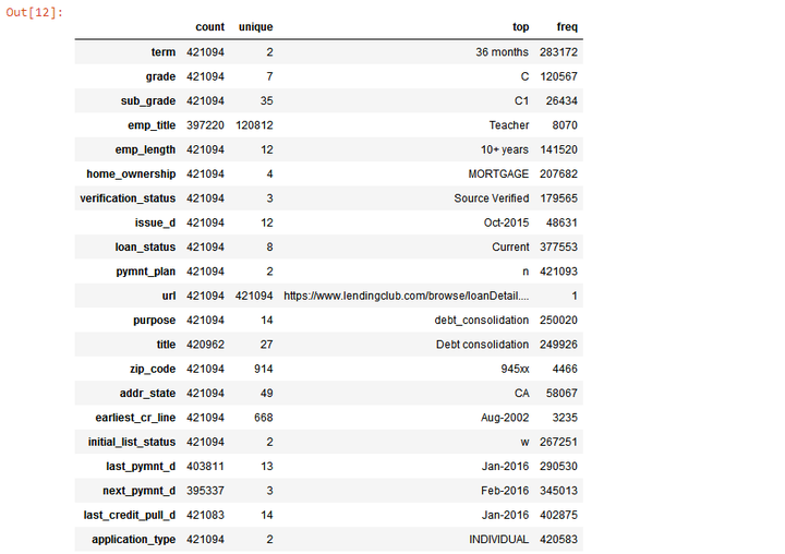
初步了解“Object”变量概况。
#初步了解“Object”变量概况
pd.set_option('display.max_rows',None)
loans.select_dtypes(include=['object']).describe().T
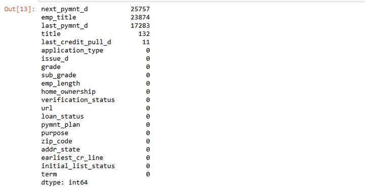
Object”分类变量缺失值概况。
#查看“Object”分类变量缺失值概况。
objectColumns = loans.select_dtypes(include=["object"]).columns
loans[objectColumns].isnull().sum().sort_values(ascending=False)
使用‘unknown’来填充缺失值。
#使用‘unknown’来填充缺失值
objectColumns = loans.select_dtypes(include=["object"]).columns # 筛选数据类型为object的数据
loans[objectColumns] = loans[objectColumns].fillna("Unknown") #以分类“Unknown”填充缺失值
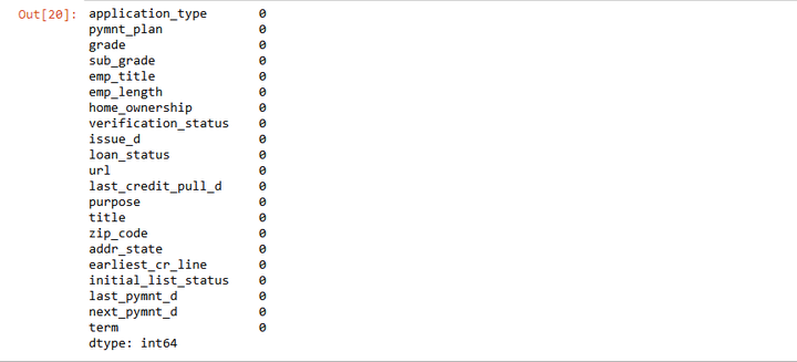
确认“Object”分类变量无缺失值。
#查看“Object”分类变量缺失值情况
loans[objectColumns].isnull().sum().sort_values(ascending=False)
处理“float64”数值型变量缺失值。
loans.select_dtypes(include=[np.number]).isnull().sum().sort_values(ascending=False)
结果发现只有两个变量存在缺失值,使用mean值来填充缺失值。
#利用sklearn模块中的Imputer模块填充缺失值
numColumns = loans.select_dtypes(include=[np.number]).columns
from sklearn.preprocessing import Imputer
imr = Imputer(missing_values='NaN', strategy='mean', axis=0)  # 针对axis=0 列来处理
imr = imr.fit(loans[numColumns])
loans[numColumns] = imr.transform(loans[numColumns])
再次查看数值变量缺失值。
loans.select_dtypes(include=[np.number]).isnull().sum().sort_values(ascending=False)
从上表中可以看到数值变量中已经没有缺失值。
本文的目的是对平台用户的贷款违约做出预测,所以需要筛选得到一些对用户违约有影响的信息,其他不相关的冗余信息,需要将其删除掉。
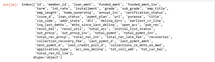
首先查看所有的分类标签
loans.columns
- sub_grade:与Grade的信息重复
- emp_title :缺失值较多,同时不能反映借款人收入或资产的真实情况
- zip_code:地址邮编,邮编显示不全,没有意义
- addr_state:申请地址所属州,不能反映借款人的偿债能力
- last_credit_pull_d :LendingClub平台最近一个提供贷款的时间,没有意义
- policy_code : 变量信息全为1
- pymnt_plan 基本是n
- title: title与purpose的信息重复,同时title的分类信息更加离散
- next_pymnt_d : 下一个付款时间,没有意义
- policy_code : 没有意义
- collection_recovery_fee: 全为0,没有意义
- earliest_cr_line : 记录的是借款人发生第一笔借款的时间
- issue_d : 贷款发行时间,这里提前向模型泄露了信息
- last_pymnt_d、collection_recovery_fee、last_pymnt_amnt: 预测贷款违约模型是贷款前的风险控制手段,这些贷后信息都会影响我们训练模型的效果,在此将这些信息删除
- url:所有的行都不同,没有分类意义
将以上重复或对构建预测模型没有意义的属性进行删除。
#删除对模型没有意义的列
loans2=loans.drop(['sub_grade', 'emp_title',  'title', 'zip_code', 'addr_state','url'], axis=1, inplace = True)
loans3=loans.drop(['issue_d', 'pymnt_plan',  'earliest_cr_line', 'initial_list_status', 'last_pymnt_d','next_pymnt_d','last_credit_pull_d'], axis=1, inplace = True)
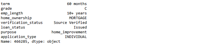
再次查看‘Object’类型变量,只剩下8个分类变量。
object_columns_df3 =loans.select_dtypes(include=["object"]) #筛选数据类型为object的变量
print(object_columns_df3.iloc[0])
数据预处理完后,接下来探索数据的特征工程,为后续的违约预测模型做好建模准备工作
特征工程是机器学习最重要的一部分,希望找到的特征是最贴近实际业务场景的,所以要反复去找特征,只需要最少的特征得到简单的模型,并且有最好的预测效果。
本节将特征工程主要分3大部分:特征抽象 、特征缩放 、特征选择
数据集中有很多的“Object”类型的分类变量存在,但是对于这种变量,机器学习算法不能识别,需要将其转化为算法能识别的数据类型。
首先对于"loan_status"数据类型转换
#统计"loan_status"数据的分布
loans['loan_status'].value_counts()
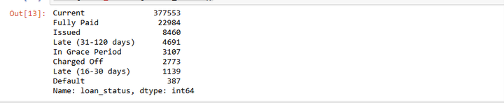
将上表中的违约编码为1,正常的为0进行编码。
#使用Pandas replace函数定义新函数:
def coding(col, codeDict):
    colCoded = pd.Series(col, copy=True)
    for key, value in codeDict.items():
        colCoded.replace(key, value, inplace=True)
    return colCoded

#把贷款状态LoanStatus编码为违约=1, 正常=0:
pd.value_counts(loans["loan_status"])
loans["loan_status"] = coding(loans["loan_status"], {'Current':0,'Fully Paid':0\
                                                     ,'In Grace Period':1\
                                                     ,'Late (31-120 days)':1\
                                                     ,'Late (16-30 days)':1\
                                                     ,'Charged Off':1\
                                                     ,"Issued":1\
                                                     ,"Default":1\
                                                    ,"Does not meet the credit policy. Status:Fully Paid":1\
                                         ,"Does not meet the credit policy. Status:Charged Off":1})

print( '\nAfter Coding:')
pd.value_counts(loans["loan_status"])
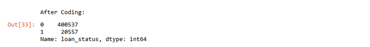
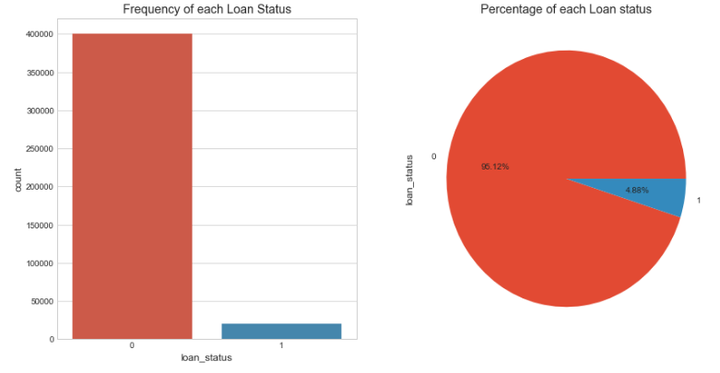
可视化查看"loan_status"中不同状态的替换情况。
# 贷款状态分布可视化
fig, axs = plt.subplots(1,2,figsize=(14,7))
sns.countplot(x='loan_status',data=loans,ax=axs[0])
axs[0].set_title("Frequency of each Loan Status")
loans['loan_status'].value_counts().plot(x=None,y=None, kind='pie', ax=axs[1],autopct='%1.2f%%')
axs[1].set_title("Percentage of each Loan status")
plt.show()
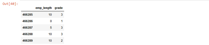
变量“emp_length”、"grade"进行特征抽象化
# 构建mapping,对有序变量"emp_length”、“grade”进行转换
mapping_dict = {
    "emp_length": {
        "10+ years": 10,
        "9 years": 9,
        "8 years": 8,
        "7 years": 7,
        "6 years": 6,
        "5 years": 5,
        "4 years": 4,
        "3 years": 3,
        "2 years": 2,
        "1 year": 1,
        "< 1 year": 0,
        "n/a": 0
    },
    "grade":{
        "A": 1,
        "B": 2,
        "C": 3,
        "D": 4,
        "E": 5,
        "F": 6,
        "G": 7
    }
}

loans = loans.replace(mapping_dict) #变量映射
loans[['emp_length','grade']].head() #查看效果
变量"home_ownership", "verification_status", "application_type","purpose", "term" 狂热编码
#变量狂热编码
n_columns = ["home_ownership", "verification_status", "application_type","purpose", "term"]
dummy_df = pd.get_dummies(loans[n_columns])# 用get_dummies进行one hot编码
loans = pd.concat([loans, dummy_df], axis=1) #当axis = 1的时候,concat就是行对齐,然后将不同列名称的两张表合并
loans = loans.drop(n_columns, axis=1)  #清除原来的分类变量
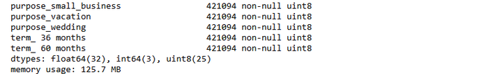
重新查看数据集中的数据类型
loans.info() #查看数据信息
采用标准化的方法进行去量纲操作,加快算法收敛速度,采用scikit-learn模块preprocessing的子模块StandardScaler进行操作。
col = loans.select_dtypes(include=['int64','float64']).columns
col = col.drop('loan_status') #剔除目标变量
loans_ml_df = loans # 复制数据至变量loans_ml_df
from sklearn.preprocessing import StandardScaler # 导入模块
sc =StandardScaler() # 初始化缩放器
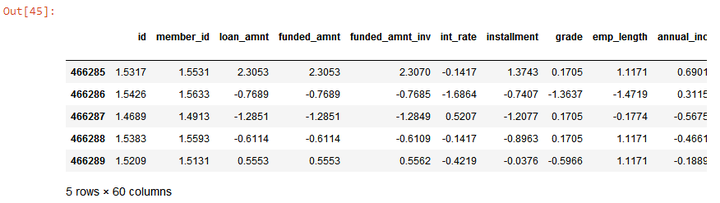
loans_ml_df[col] =sc.fit_transform(loans_ml_df[col]) #对数据进行标准化
loans_ml_df.head() #查看经标准化后的数据
以上过程完成了非数值型特征抽象化处理,使得算法能理解数据集中的数据,这么多的特征,究竟哪些特征对预测结果影响较大,所以以下通过影响大小对特征进行选择。
特征的选择优先选取与预测目标相关性较高的特征,不相关特征可能会降低分类的准确率,因此为了增强模型的泛化能力,我们需要从原有特征集合中挑选出最佳的部分特征,并且降低学习的难度,能够简化分类器的计算,同时帮助了解分类问题的因果关系。
一般来说,根据特征选择的思路将特征选择分为3种方法:嵌入方法(embedded approach)、过滤方法(filter approach)、包装方法(wrapper approacch)。
- 过滤方法(filter approach): 通过自变量之间或自变量与目标变量之间的关联关系选择特征。
- 嵌入方法(embedded approach): 通过学习器自身自动选择特征。
- 包装方法(wrapper approacch): 通过目标函数(AUC/MSE)来决定是否加入一个变量。
本次项目采用Filter、Embedded和Wrapper三种方法组合进行特征选择。
首先将数据集中的贷款状态'loan_status'抽离出来
#构建X特征变量和Y目标变量
x_feature = list(loans_ml_df.columns)
x_feature.remove('loan_status')
x_val = loans_ml_df[x_feature]
y_val = loans_ml_df['loan_status']
len(x_feature) # 查看初始特征集合的数量

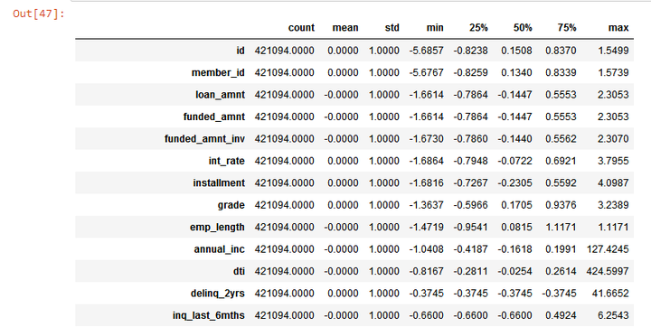
重新查看没有贷款状态'loan_status'的数据集。
x_val.describe().T # 初览数据
Wrapper方法
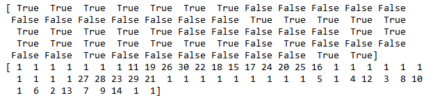
选出与目标变量相关性较高的特征。通过暴力的递归特征消除 (Recursive Feature Elimination)方法筛选30个与目标变量相关性最强的特征,将特征维度从59个降到30个。
from sklearn.feature_selection import RFE
from sklearn.linear_model import LogisticRegression
# 建立逻辑回归分类器
model = LogisticRegression()
# 建立递归特征消除筛选器
rfe = RFE(model, 30) #通过递归选择特征,选择30个特征
rfe = rfe.fit(x_val, y_val)
# 打印筛选结果
print(rfe.support_)
print(rfe.ranking_) #ranking 为 1代表被选中,其他则未被代表未被选中
通过布尔值筛选首次降维后的变量。
col_filter = x_val.columns[rfe.support_] #通过布尔值筛选首次降维后的变量
col_filter # 查看通过递归特征消除法筛选的变量
Filter方法
正常情况下,影响目标变量的因数是多元性的;但不同因数之间会互相影响(共线性 ),或相重叠,进而影响到统计结果的真实性。下一步,以下通过皮尔森相关性图谱找出冗余特征并将其剔除,且通过相关性图谱进一步引导我们选择特征的方向。
colormap = plt.cm.viridis
plt.figure(figsize=(12,12))
plt.title('Pearson Correlation of Features', y=1.05, size=15)
sns.heatmap(loans_ml_df[col_filter].corr(),linewidths=0.1,vmax=1.0, square=True, cmap=colormap, linecolor='white', annot=True)
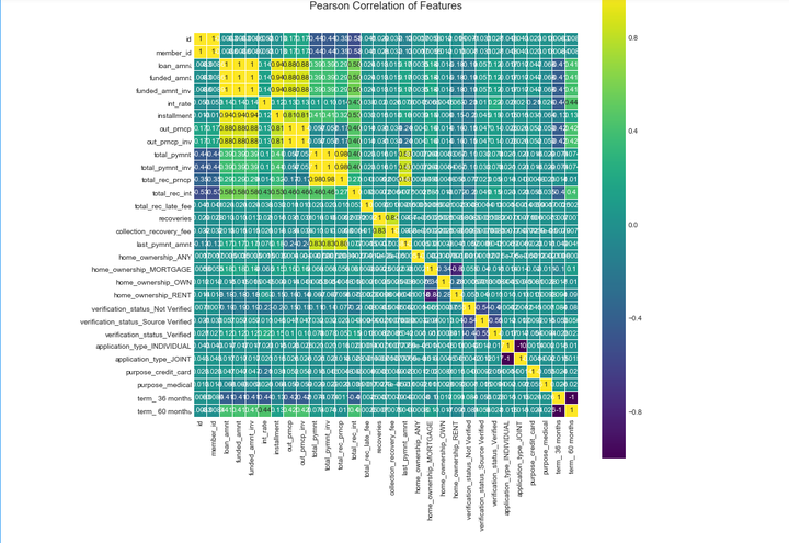
从上图中得到需要删除的冗余特征。
drop_col = ['id','member_id','collection_recovery_fee','funded_amnt', 'funded_amnt_inv','installment', 'out_prncp', 'out_prncp_inv',
                       'total_pymnt_inv', 'total_rec_prncp', 'total_rec_int', 'home_ownership_OWN',
                       'application_type_JOINT',  'home_ownership_RENT' ,
                       'term_ 36 months', 'total_pymnt', 'verification_status_Source Verified', 'purpose_credit_card','int_rate']
col_new = col_filter.drop(drop_col) #剔除冗余特征
print(len(col_new))

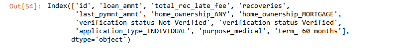
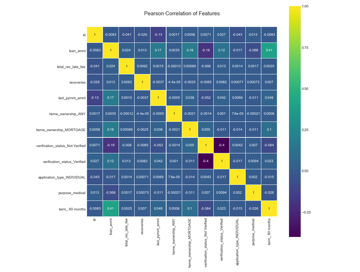
特征从30个降到12个,再次确认处理后的数据相关性。
col_new # 查看剩余的特征
colormap = plt.cm.viridis
plt.figure(figsize=(12,12))
plt.title('Pearson Correlation of Features', y=1.05, size=15)
sns.heatmap(loans_ml_df[col_new].corr(),linewidths=0.1,vmax=1.0, square=True, cmap=colormap, linecolor='white', annot=True)
Embedded方法
为了了解每个特征对贷款违约预测的影响程度,所以在进行模型训练之前,我们需要对特征的权重有一个正确的评判和排序,就可以通过特征重要性排序来挖掘哪些变量是比较重要的,降低学习难度,最终达到优化模型计算的目的
#随机森林算法判定特征的重要性
names = loans_ml_df[col_new].columns
from sklearn.ensemble import RandomForestClassifier
clf=RandomForestClassifier(n_estimators=10,random_state=123)#构建分类随机森林分类器
clf.fit(x_val[col_new], y_val) #对自变量和因变量进行拟合
names, clf.feature_importances_
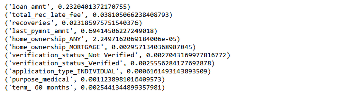
for feature in zip(names, clf.feature_importances_):
print(feature)
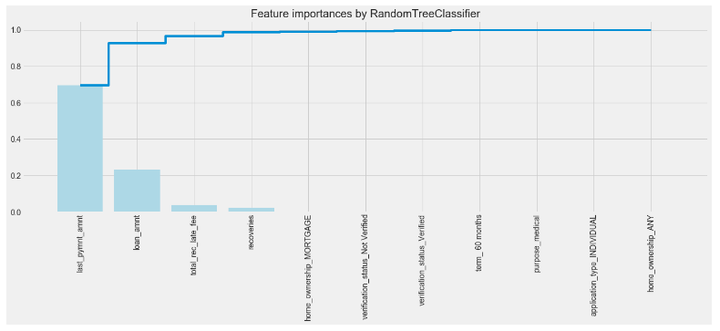
特征重要性从大到小排序及可视化图形,结果发现最具判别效果的特征是收到的最后付款总额‘last_pymnt_amnt’
本项目中,2015年度贷款平台上违约的借款人比例很低,约为4.9%,正负样本量非常不平衡,非平衡样本常用的解决方式有2种:
-
过采样(oversampling),增加正样本使得正、负样本数目接近,然后再进行学习。
-
欠采样(undersampling),去除一些负样本使得正、负样本数目接近,然后再进行学习。
#构建自变量和因变量
X = loans_ml_df[col_new]
y = loans_ml_df["loan_status"]
n_sample = y.shape[0]
n_pos_sample = y[y == 0].shape[0]
n_neg_sample = y[y == 1].shape[0]
print('样本个数:{}; 正样本占{:.2%}; 负样本占{:.2%}'.format(n_sample,
	   n_pos_sample / n_sample,
	   n_neg_sample / n_sample))
print('特征维数:', X.shape[1])

from imblearn.over_sampling import SMOTE # 导入SMOTE算法模块
# 处理不平衡数据
sm = SMOTE(random_state=42)    # 处理过采样的方法
X, y = sm.fit_sample(X, y)
print('通过SMOTE方法平衡正负样本后')
n_sample = y.shape[0]
n_pos_sample = y[y == 0].shape[0]
n_neg_sample = y[y == 1].shape[0]
print('样本个数:{}; 正样本占{:.2%}; 负样本占{:.2%}'.format(n_sample,
                                                   n_pos_sample / n_sample,
                                                   n_neg_sample / n_sample))

采用逻辑回归分类器 分类器进行训练
# 构建逻辑回归分类器
from sklearn.linear_model import LogisticRegression
clf1 = LogisticRegression()
clf1.fit(X, y)
查看预测结果的准确率
predicted1 = clf.predict(X) # 通过分类器产生预测结果
from sklearn.metrics import accuracy_score
print("Test set accuracy score: {:.5f}".format(accuracy_score(predicted1, y,)))

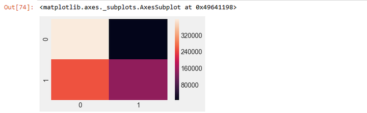
利用混淆矩阵及可视化观察预测结果
#生成混淆矩阵
from sklearn.metrics import confusion_matrix
confusion_matrix(y, predicted1)

# 混淆矩阵可视化
plt.figure(figsize=(5,3))
sns.heatmap(m)
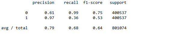
再利用sklearn.metrics子模块classification_report查看precision、recall、f1-score的值
#查看precision、recall、f1-score的值
from sklearn.metrics import classification_report
print(classification_report(y, predicted1))
#计算ROC值
from sklearn.metrics import roc_auc_score
roc_auc1 = roc_auc_score(y, predicted1)
print("Area under the ROC curve : %f" % roc_auc1)

以上完成了全部的模型训练及预测工作。
本文基于互联网金融平台2015年度贷款数据完成信贷违约预测模型,全文包括了数据清洗,构建特征工程,训练模型,最后得到的模型准确率达到了0.79,召回率达到了0.68,具有较好的预测性,本文的模型可以作为信贷平台预测违约借款人的参考

