fani-lab / adila Goto Github PK

Summary:
While running the det_cons algorithm on random baseline, I received a Key Error. After tracing back, we figured out in the self.data dictionary (reranking -> algs.py -> line 232) the index of popular users exceeds their size and we get key error.
We believe this is due to the popular/non-popular ratio that we pass to the reranker (Popular: 0.43999999999999995, Non-popular: 0.56). Other ratios or other values of k_max might bypass this error if the required number of experts per each group does not exceed their availability.

Run Settings:
prediction file that caused the issue: title.basics.tsv.filtered.mt75.ts3/random/t32059.s23.m2011.b4096/f0.test.pred

re-ranking algorithm: det_cons

k_max: size of the team (2011 experts)

ratio: {True: 0.43999999999999995, False: 0.56}

splits: title.basics.tsv.filtered.mt75.ts3/splits.json

teamsvec file : title.basics.tsv.filtered.mt75.ts3/teamsvecs.pkl

Traceback:

Traceback (most recent call last):
  File "C:/Users/Hamed/AppData/Local/JetBrains/Toolbox/apps/PyCharm-P/ch-0/222.3739.56/plugins/python/helpers/pydev/pydevd.py", line 1496, in _exec
    pydev_imports.execfile(file, globals, locals)  # execute the script
  File "C:\Users\Hamed\AppData\Local\JetBrains\Toolbox\apps\PyCharm-P\ch-0\222.3739.56\plugins\python\helpers\pydev\_pydev_imps\_pydev_execfile.py", line 18, in execfile
    exec(compile(contents+"\n", file, 'exec'), glob, loc)
  File "C:/Projects/Equality/src/main.py", line 348, in <module>
    utility_metrics=args.utility_metrics)
  File "C:/Projects/Equality/src/main.py", line 242, in run
    reranked_idx, probs, elapsed_time = Reranking.rerank(preds, labels, new_output, ratios, algorithm, k_max, cutoff)
  File "C:/Projects/Equality/src/main.py", line 102, in rerank
    algorithm=algorithm)
  File "C:\Projects\Equality\env\lib\site-packages\reranking\__init__.py", line 18, in rerank
    return rerank(k_max, algorithm, verbose)
  File "C:\Projects\Equality\env\lib\site-packages\reranking\algs.py", line 80, in __call__
    return self.rerank_greedy(k_max_, algorithm, verbose)
  File "C:\Projects\Equality\env\lib\site-packages\reranking\algs.py", line 232, in rerank_greedy
    re_ranked_ranking.append(self.data[(next_attr, counts[next_attr])])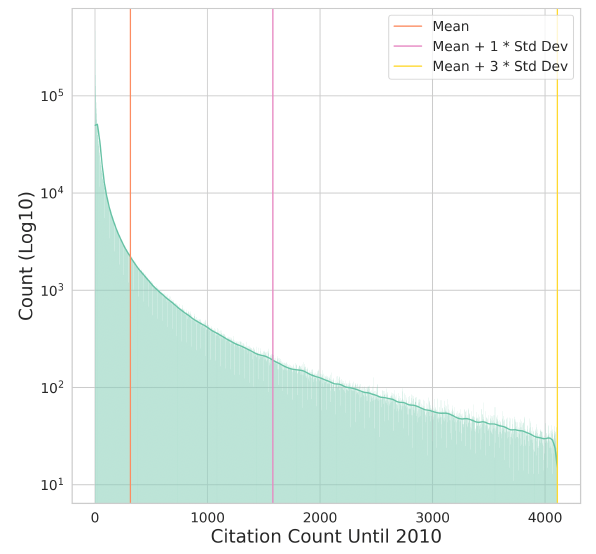
KeyError: (0, 856)

We need to justify the threshold of being popular vs. nonpopular based on distribution of experts.
1- We need a figure that shows the distribution and draw the lines on it to show the mean, mean+1std, mean+2std, ... with the value annotated on the lines. Something like this:

2- We need another figure that shows the area under the curve of distribution and split that area into two equal size, annotating each area with the same number. Something like this.

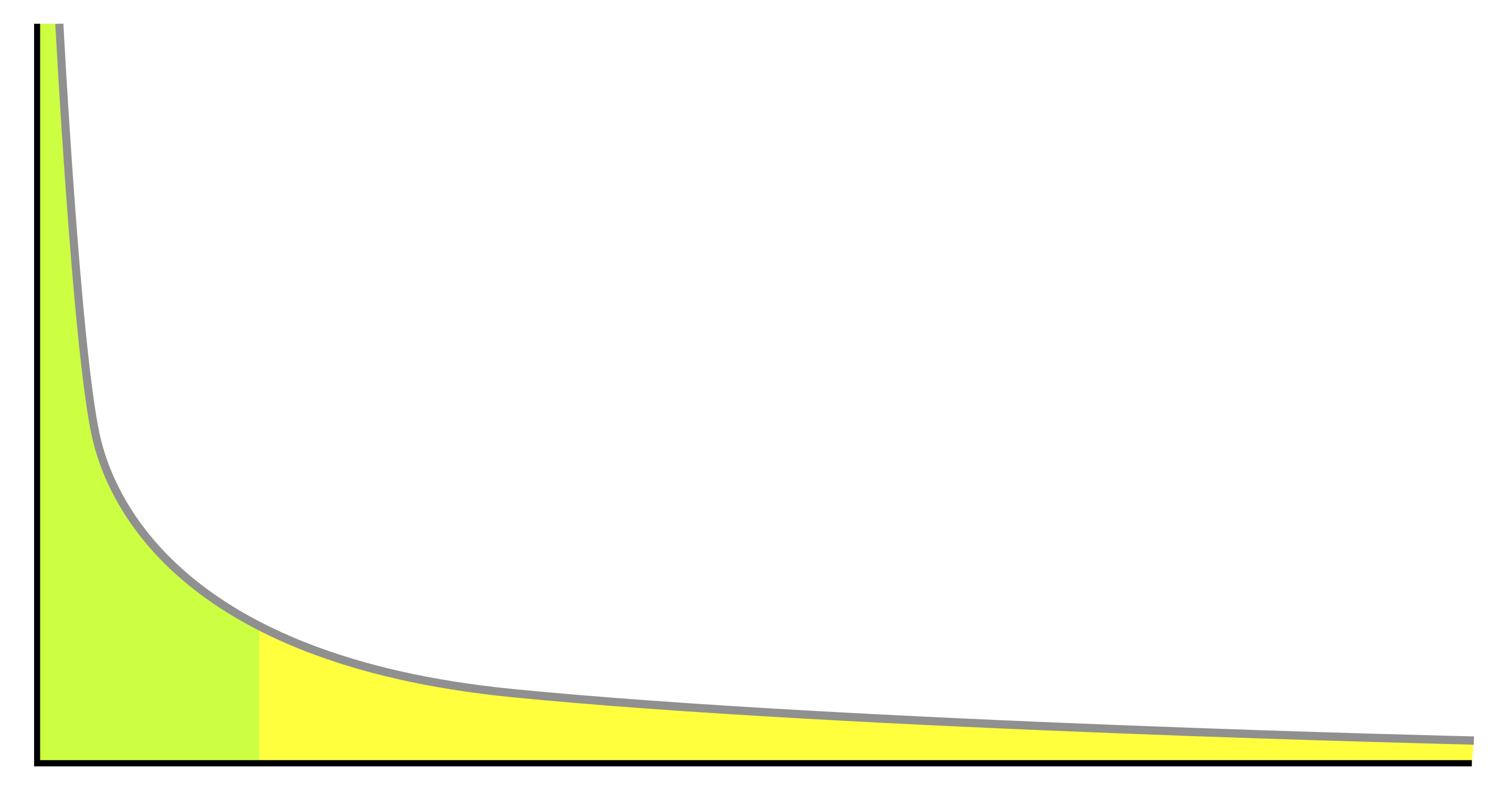
Hopefully, the mean and the area of splited under the carve are close.

@Hamedloghmani @edwinpaul121
How about this issue as the next task for Edwin?

@Hamedloghmani
When running Adila in parallel for multiple *.pred files, we rely on file locking system of os. However, there will be some issues like

One process may be true in condition check, but when creating see the folder exists due to other process!

Or when logging the time at:

Temporary solution is to run sequentially for one pred file. Then, run in parallel for all files.

Today I have been struggling with this issue while trying to run my experiment for double cutoff method based on the refactored code. NDKL is always zero for every input.
I am prioritizing the task of resolving this bug.

An ad hoc team is one where the agents in the team have not collaborated with each other [Weighted synergy graphs for effective team formation with heterogeneous ad-hoc agents: Somchaya & Manuela].

• Find papers/movies/patents/.. whose members are not part of previous papers => those teams whose members meet for the first time (the first joint collaboration)

This is the second step of mitigating the popularity bias using a reranking method.

We are going to see the distribution of genders over inventors in uspt dataset

Hello @edwinpaul121

This is your first task and issue page in this project, welcome 😄

Your task is to design and implement a function to create a bubble plot from 2 given list of float numbers. One of these lists is fairness, the other one is utility. Consider the lists have the same length.

Please try to write the function as generic as possible as we discussed and include other necessary arguments to customize the plot.
Some bubble plot samples can be found here

You can log your progress and problems here. Please let me know if you have any questions.

Thanks

In Adila, we are using torch library just to load our .pred files. Using just a small function from a big toolkit is not desirable since being lightweight is one of our goals in Adila's development. We are looking for an alternate tool to remove torch from pipeline and use that library or toolkit instead for loading .pred files. Note that .pred files are PyTorch model predictions (e.g outputs of OpeNTF).

This issue is regarding the process of adding the equal area under curve plot feature to the pipeline
A sample is shown below:

Problem:

Our results in ECIR-Bias2023 (issue #34) suggest that deterministic greedy re-ranking algorithms are not successful in avoiding utility loss while maintaining fairness in different teams.

Proposed Solution:

Our proposed solutions for this was the double-cutoff method that I'll explain with an example.
Suppose we need a team of 5 experts and we have the output by the size of 20 from the team formation baseline. Instead of passing 20 people to re-ranker, we first sort them by probability/score, select the top 10, then pass those to the re-ranker algorithm with k=5. We were planning to keep less related individuals out of the re-ranker's reach.

Causes of Failure

This attempt was not successful since the main cause of utility loss was sparsity of our search space compared to the search space that these algorithms were originally developed on. Det_greedy, det_cons and det_relaxed work in an iterative manner and in each iteration they select the expert with highest popularity/score from the set of experts with under represented sensitive attribute. Hence, our solution was not helpful for this issue.
The sparsity problem will be more clear after finishing our analysis on other datasets and search spaces (#40)

This issue breaks down the required steps to implement equality of opportunity fairness criteria in Adila.

• 1. in this step we try to find a matrix that show which members had each of the skills. To do so we should do the following
  teamids, skillvecs, membervecs = teamsvecs['id'], teamsvecs['skill'], teamsvecs['member']
skill_member = skillvecs.transpose() @ membervecs
  in skill_member, rows would be skills and columns would be members

• 2. For each team, we find the required skills

• 3. Find the qualified set ( set of members that have all the required skills for the team)

• 4. Extract Popular vs Non-popular in qualified set and pass to re-ranker

Questions before the final implementation:

1. Which part of the pipeline is the correct spot to put this implementation (obviously should be before rerankfunction)?
2. Does row id in .pred files represent teamids in teamsvec file ?

Title: Debiasing the Human-Recommender System Feedback Loop in Collaborative Filtering

Venue: (WWW ’19 Companion) San Francisco, CA, USA

Year: 2019

main problem
Recommendation system introduce a phenomenon called as ‘filter bubble’. A situation where users only see a narrow subset of the entire range of available recommendations. Recommendation systems biggest problem is, it knows why a user likes an item, it doesn’t know why an item is not-liked by the user

input
A Rating matrix Ru′ i, λ, Learning rate η, MAXinteration, Iterations=0, Sizeofselection

Output
Mean Absolute error, Root mean square error, Gini coefficient
The system trains the initial Matrix Factorization model and computes predictions Rˆ


Motivation
Introducing debasing algorithms for Recommendation systems based on Matrix factorization during the chain of events in which users actively interact with Recommendation systems

Previous Works and their Gaps

• an implicit feedback model to measure the level of confidence that a user will see an item
• Schnabel introduced recommending items in an RS is analogous to exposing a patient to a randomized treatment in a medical study, and proposed the introduction of a propensity-scored recommendation learning system
• Chanely et al. observed that algorithms increase homogeneity among users, thereby decreasing the utility gained by users of the system, and presented a simulation to illustrate how this effect occurs

Contributions

• a unified recommendation and active learning strategy (active recommendation) during the interaction between users and the RS
• an exposure-based collaborative filtering recommendation model that is also combined with an active recommendation to further debias the RS
• a blind spot aware MF, which takes into account the blind spot inherent in the learning phase of the RS. 4.

Proposed Method
randomly select 25 items for each of the 500 users from the completed rating matrix and start the initial training. Later on they select 20% of the ratings as the test set. This testing set is later fixed, All other ratings are considered candidate ratings: they are used to simulate the feedback loop of Recommendation system and human interaction. In each feedback loop they implement one of the algorithms to recommend items to each user to which the response is simulated

Experiments
An item response theory to generate a sparse rating matrix using the model proposed in the paper 'Rank aggregation via nuclear norm minimization' (https://arxiv.org/pdf/1102.4821.pdf) .
A dataset is generate with a rating matrix R with 500 users and 500 items, total of 250,000 ratings

code
https://github.com/wenlong-sun7/Debiasing-the-Human-Recommender-System-Feedback-Loop-in-Collaborative-Filtering

Gaps of this work
assuming that users totally agree with the recommendations in each iteration, and provide feedback.

Fairness 1: Fair distribution of stars in all teams #6
Fairness 2: Equal number of each class #5
Fairness 3: Lack of discrimination (bias) #18

Since this paper had a lot of mathematical equations and terms, I had to attach a pdf version of my summary because the editor here does not support a lot of features eg. subscript or superscript. Sorry for the inconvenience this may cause.
2022-SIGIR-Bilateral Self-unbiased Learning from Biased Implicit Feedback.pdf

Hi @hosseinfani
When I tried to load the recent pickle file for Teamsvec from OpenTF version 0.1 and 0.2. I ran into an error:

This is not a common error at all. Finally I found the error, and the solution here:
RasaHQ/rasa#10908 (comment)

Basically, everything trained and saved using scipy version 1.8 or greater, will be incompatible in the production phase. The only provided solution that I saw was downgrading scipy, re-training the model (OpenTF) and get the results again.

First, we have to start with the application of propensity score and when it should be utilized. Propensity score analysis is a class of statistical methods developed for estimating treatment effects with nonexperimental or observational data. Specifically, propensity score analysis offers an approach to program evaluation when randomized trials are infeasible or unethical, or when researchers need to assess treatment effects from survey data, census data, administrative data, medical records data, or other types of data “collected through the observation of systems as they operate in normal practice without any interventions implemented by randomized assignment rules” (Rubin, 1997,p. 757). In the social and health sciences, researchers often face a fundamental task of drawing conditioned casual inferences from quasi-experimental studies. Analytical challenges in making causal inferences can be addressed by a variety of statistical methods, including a range of new approaches emerging in the field of propensity score analysis. As a new and rapidly growing class of evaluation methods, propensity score analysis is by no means conceived as the best alternative to randomized experiments. In empirical research, it is still unknown under what circumstances the approach appears to reduce selection bias and under what circumstances the conventional regression approach (i.e., use of statistical controls) remains adequate. However, it is also a consensus among prominent researchers that the propensity score approach has reached a mature level.

To define the propensity score, we introduce the following notation: let X=(X1,..,Xn) represent confounders that are measured prior to intervention initiation (referred as “baseline confounders” below), then X=(X1i,..,Xni) is a vector of the value of the n confounders for the ith subject. Let n represent the available interventions, with T=1 indicating the subject is in the treated group and T=0 meaning the subject in the control group. For the ith subject, the propensity score is the conditional probability of being in the treated group given their measured baseline confounders,
p(Xi) = Prob( Ti = 1|Xi)

Intuitively, conditioning on the propensity score, each subject has the same chance of receiving treatment. Thus, propensity score is a tool to mimic randomization when randomization is not available.
In other words, A propensity score is the probability of a unit (e.g., person, classroom, school) being assigned to a particular treatment given a set of observed covariates. Propensity scores are used to reduce selection bias by equating groups based on these covariates. Suppose that we have a binary treatment indicator Z, a response variable r, and background observed covariates X. The propensity score is defined as the conditional probability of treatment given background variables:
e(x) = Prob( Z = 1| X=x)

Side Note:

• Confounders: In statistics, a confounder is a variable that influences both the dependent variable and independent variable, causing a spurious association.

• Binary Treatment Indicator: the treatment can be written as a variable T:1. Ti = { 1 if unit i receives the “treatment” 0 if unit i receives the “control”}

• Response Variable: A variable is a covariate if it is related to the dependent variable. According to this definition, any variable that is measurable and considered to have a statistical relationship with the dependent variable would qualify as a potential covariate.

References:
[1] Guo, Shenyang, and Mark W. Fraser. Propensity score analysis: Statistical methods and applications. Vol. 11. SAGE publications, 2014.
[2] Faries, Douglas, et al. Real world health care data analysis: causal methods and implementation using SAS. SAS Institute, 2020.
[3] Van der Laan, Mark J., and Sherri Rose. Targeted learning: causal inference for observational and experimental data. Vol. 10. New York: Springer, 2011.

Title: FA*IR: A Fair Top-k Ranking Algorithm
Year: 2017
Venue: CIKM

Main Problem:
Formal problem of Fair top-k ranking is formally defined as follows(notation is adapted from paper):
Given a set of candidates, we want to produce a ranking that satisfies following conditions:
(i) satisfies the in-group monotonicity constraint
The requirement of in-group monotonicity constraints applies to all individuals and mandates that both candidates who are protected and those who are not, should be arranged in descending order of qualifications(qualification is considered as each member's utility or score in this paper) separately.
(ii) satisfies ranked group fairness
It means every prefix of the ranking should satisfy group fairness condition which is presence of specific amount of protected groups in the ranking
(iii) achieves optimal selection utility subject to (i) and (ii)
It means we prefer rankings in which the more qualified candidates are included, and the less qualified ones are excluded.
(iv) maximizes ordering utility subject to (i), (ii), and (iii).
It means a ranking should be ordered by decreasing qualification.

To summarize, we need a ranking that 1) fairly represent protected group(we define the percentage), 2) contain most qualified members based the obtained score from a machine learning model or score function and 3) ranking should be ordered by decreasing qualification

Drawbacks of Related Work
This paper is one of the early attempts for algorithmic fair ranking. Hence, there were no rich body of baselines to compare. They mentioned a constraint based optimization fair ranking method [1]. The problem of the construction of the constraint matrix was left open in that work and it is addressed in this paper.

Proposed Method
Input:

• the expected size k of the ranking to be returned
• the qualifications (or scores, probabilities, etc.)
• protected attribute labels (popularity labels for example)
• minimum proportion of the protected group
• adjusted significance level

Output: a ranking of size k

First, the algorithm creates two priority queues, one for each protected group ( e.g. 1 for popular member 1 for nonpopular ones). Then based on the desired distribution, algorithm creates a table ( this table is stored for time efficiency). In this table it is mentioned that for each prefix of the ranking with size o < k, what is the minimum number of required members from the protected group. Then it greedily and iteratively constructs a ranking subject to candidate qualifications, and minimum protected members required. For each position in each iteration, if we need protected member, the one with best qualification is selected. Otherwise the best member from their union is selected. A sample of this table is as follows:

Results and Conclusion
Their approach has the ability to produce a ranking that ensures fairness among ranked groups, and their experiment indicates that it does not result in a significant loss of utility metrics( in their case NDCG). In comparison to the method proposed by Feldman et al., their approach typically results in the same or lower loss of utility. Also, they do not make the assumption that the qualification distributions in the protected and non-protected groups are identical in shape. Most importantly, they can regulate the trade-off between fairness and utility through a parameter, p (or known as p-value).

Limitations:

• They only had 2 other baselines in their comparison. First, color blind ranking which is ranking without fairness considerations just based on utility. Second, Feldman et al., which aligns the probability distribution of the protected candidates with the non-protected ones.
• Their method only supports one protected attribute with binary value. ( It is notable that the same authors addressed this issue in their future papers)

Datasets:

• COMPAS
• German Credit
• SAT Score Dataset 2014
• XING Dataset (proposed with this paper) : a career-oriented website like LinkedIn talent.

Codebase:
https://github.com/MilkaLichtblau/FA-IR_Ranking

References:
[1] L Elisa Celis, Damian Straszak, and Nisheeth K Vishnoi. 2017. Ranking with Fairness Constraints. arXiv:1704.06840 (2017).

Please provide some info about this dataset, paper, ... and link the summary (issue) to this issue.

Title: Fairness-Aware Ranking in Search & Recommendation Systems with application to LinkedIn Talent Search
Year: 2019
Venue: KDD

Main Problem:
Generally, when we are ranking people in real life, many factors might be the potential source of bias in the process of our decision such as looks, gender, behavior etc. The same issue is relatable in machine learning based decision making in ranking people and team formation. This problem can be tackled by three main approaches. First, by pre-processing which means the efforts before the training process such as dataset creation or feature engineering. Second, modifications dedicated to the model. And finally, post processing which includes calibrating the output of a potentially biased system in order to get unbiased results. This paper authors focused on the last approach.

Proposed Method:
In order to make fairness definition more formal, they defined two conditions (original numbering is kept for ease):

r: A search request or a recommendation task
A = {a1, . . ., al}: Set of disjoint protected attribute values (each candidate has exactly one value in A); Note that we denote the attribute value for candidate x as A (x), by abuse of notation. τr : Ranked list of candidates for r; τr [j] denotes jth candidate; τr k denotes the first k candidates in τr
pq,r,ai : Desired proportion of candidates with attribute value ai that should be in the ranked list pτr ,r,ai : Proportion of candidates in τr with value ai
count k (ai) denotes the number of candidates with attribute value ai among the top k results

The second condition is more important since it makes sure an attribute has at least the minimum representation that we expect.
The authors came up with four different ranking algorithms. DetGreedy is an algorithm that first checks if any attribute is going to break the constraint #6, if so, it will choose the one with the highest score among them. Otherwise, the attribute with the highest next score from the list of attributes that have not satisfied their maximum requirement will be picked.
DetCons and DetRelaxed: The authors propose these algorithms while pointing out that the previous one will easily fall into infeasible state. Their first step is just like the previous algorithm but if constraint #6 is not going to be violated, they favor one for the attributes that their minimum representation requirement is likely to be violated soon in the ranking.
It is notable that “the above algorithms are feasible when the number of possible attribute values for protected attribute is less than 4.”
DetConSort can be considered as a method to solve a general interval constrained sorting problem and the objective function is the maximization of the sorting quality.
They argued that there is no single best algorithm and there is always a trade-off between utility and fairness.
Dataset:
Instead of using a dataset they used simulation because of two reasons. First, to be able to study settings where there could be several possible values for the protected attribute. Second, avoiding the challenge of position bias. In terms of fairness literature, the equalized odds metric is addressed in this work.

Input and Output:

Gaps:

1. Authors could not prove that the algorithms are feasible all the time.
2. The propossed methods are problem-specific. Taking the approaches that modifies the training process will be more generalizable.
3. They defined a fairness metric and measured fairness with it without proving how effective this measure would be in case of finding bias.

Codebase ( unofficial):
https://github.com/yuanlonghao/reranking

FAIRNESS AND MACHINE LEARNING BOOK
Limitations and Opportunities
Solon Barocas, Moritz Hardt, Arvind Narayanan

Summary 1

Recommended by: Benjamin Fish

Title: Measuring Fairness in Ranked Outputs
Year: 2017
Venue: SSDBM

My notes:
One of the main challenges that I faced during experimenting on fairness in ranking was lack of proper metric to measure fairness. To the best of my knowledge, the following paper proposed three metrics to measure fairness specifically for ranking. Although 6 years have passed since this paper, still I have not seen a fairness metric for ranking become common in literature except NDKL which is also the contribution of this paper.

Main Problem:
This paper addresses the impact of algorithmic decisions that involve scoring and ranking individuals. These decisions have significant consequences, as they determine outcomes such as credit worthiness, college admissions etc. The paper focuses specifically on situations where an institution, referred to as a "ranker," assesses a set of items, typically individuals, based on different characteristics such as demographics or behaviors. The ranker generates a ranking that represents the relative quality of these items. However, despite the seemingly objective nature of automated rankers, they can exhibit discriminatory behavior against individuals and systematically disadvantage protected groups. Moreover, lack of diversity can be observed in higher-ranking positions. Given these concerns, the authors emphasizes the need to study the fairness of ranking schemes. Fairness is broadly defined as the impartial and just treatment of individuals and demographic groups. While algorithmic fairness has gained increasing attention in literature, and numerous interpretations and technical definitions have been proposed, the authors note a lack of work quantifying fairness specifically in the context of ranking schemes. Specifically, they claim "despite a recent spike of interest in fairness, and despite the ubiquity and the importance of ranking, we are not aware of work that quantifies fairness in a ranking scheme". Therefore, the main objective of the paper is to address this research gap and provide a metric of fairness in ranking schemes.

Proposed Method:
Their approach to fairness measures is based on some concept: Since it is more advantageous for an item to have a higher rank, achieving statistical parity at higher ranks becomes more crucial. To incorporate this idea, they adopt several established statistical parity measures proposed in existing literature and integrate them into the nDCG framework. Specifically, they compute set-wise parity at multiple cutoff points within a ranking and progressively aggregate these values using a position-based discount. To keep this summary short and readable, I skip NDKL since we already know the details about that metric.

Normalized discounted difference (rND): " computes the difference in the proportion of members of the protected group at top-i and in the over-all population."

in the formula, Z is the normalization variable to determine the highest possible value for the metric (typically they keep it between 0 and 1). S+ is the protected group ( for example non-popular group in our initial experiments) and N is size of the whole set. They experimented with these metrics on a synthetic dataset to have control over the unfairness of the data over the experiment. They made some observations about this metric that I'll summarize: the protected and non-protected groups were treated symmetrically. It means low proportion of both protected or non-protected group at high ranks leads to a high (unfair) rND score. rND is convex and continuous but is not differentiable at 0.

Drawback:
While the metric is convex and continuous, it is not differentiable, limiting its usefulness in an optimization framework.

Normalized discounted ratio (rRD):
This metric is formulated similarly to rND, with the difference in the denominator of the fractions.

In the first fraction they use |S-| which is size of non-protected samples in the given range (1 to i) as the denominator and in the second fraction they used size of the whole set of non-protected group as the denominator. They mentioned: " When either the numerator or the denominator of a fraction is 0, we set the value of the fraction to 0."
Observation summary: They observe that rRD reaches its best (lowest) value at the same points as do rND and NDKL( aka rKL), but that it shows different trends. Since rRD does not treat protected and non-protected groups symmetrically, its behavior when protected group represents the majority of the over-all population or when protected group is preferred to non-protected group(fairness probability > 0.5), is not meaningful which is a negative point.

Drawback:
This metric is only applicable when the protected group(e.g non-popular group) is the minority group.

The following is the plot of all three metrics on the synthetic dataset:

Codebase:
https://github.com/DataResponsibly/FairRank/

Systems

This issue is just a log file of my progress in reviewing the sigir_2022_BISER repo.

After running the given examples for the first time. My initial thoughts is that the code is not really user friendly and understandable on first attempts. Lacks a lot of comments and even some of the comments are in Korean I guess. There were some points that was kind of surprising since this repo is the official codebase for SIGIR 2022 accepted paper.

1. Inconsistency in the material for creating an environment.

2. Using Tensorflow 1.* in a code developed in 2021-22.

3. Lack of proper comments and explanation in this code.

4. Some small issues like importing a library and not using it.

A snap shot of the first run:

Title: Fair ranking: a critical review, challenges, and future directions
Year: 2022
Venue: FAccT

This paper investigates whether, after significant research about fairness in the recommender systems literature in the past few years, we have a practical solution for fairness. Furthermore, if we do not, what are the causes? How they can be addressed.
The literature mainly focuses on the fairness of a single instance in the ranking or multiple independent instances of ranking with an additive objective across samples. Fair ranking algorithms mostly try to abstract away some of the context specifics under a reducibility assumption. For example, they look at the fair ranking problem as a typical ranking problem with some constraints regarding fairness or optimizing a (or some) suitable fairness measure. However, in [1], it is stated that this often “renders technical interventions ineffective, inaccurate, and sometimes dangerously misguided.”
There are three main classes of ways that this reduction abstracts a significant amount of the essential aspects in the fair ranking context. Those are summarized on the left side of the figure above.
In my opinion, the most prominent issues about spillover effects are: 1) ranking systems are not stand-alone products. The presence of other associated services like sponsored advertisements causes the user’s attention to spill over to other items. 2) there are competition and cross-platform spillover effects. Users may reach an item not through the recommendation engine on the platform but by means of a search engine, product or price comparison sites, or social media.
In the case of strategic behavior, current fair ranking mechanisms usually fail to take into account the fact that the providers could be strategic players who might try to actively maximize their utilities, like influencers on social media who try to jack trends. If we are planning to use such a ranking system in the real world, we must consider this issue.
Consequences of Uncertainty is the issue that the work that I recently summarized [2] tried to tackle. Current fair ranking mechanisms assume the availability of the demographic data of individuals to be ranked. These assumptions help algorithmic developments for fair ranking, but the availability of demographic data cannot be guaranteed. Uncertainties may be differential, affecting some participants more than others, even within the same protected groups. Such differential informativeness, for example, “might occur in ranking settings where the platform has more information on some participants (through longer histories, or other access differences) than others. The result of such differential informativeness may cause downstream disparate impact, such as privileging longer-serving providers over newer and smaller ones.”
However, the uncertainty remains an open question due to the complex nature of this phenomenon and various situations of happening.
Legal and Data Bottlenecks are essential issues in this area, but they do not concern our research at the moment.
My Final Conclusions:
• Fairness in ranking has a long way to go to become mature and practical. Most of the results that the methods in the literature get are in an isolated or simulation environment.
• The fairness method might even make a situation worse in terms of fairness in a real-world application if the issues above are not addressed.
• The paper was well-written and dense. It had many examples for each scenario, and I am happy with the fact that I read it (it was worth the time)

References
[1] Andrew D. Selbst, Danah Boyd, Sorelle A. Friedler, Suresh Venkatasubramanian, and Janet Vertesi. 2018. Fairness and Abstraction in Sociotechnical Systems. In ACM Conference on Fairness, Accountability, and Transparency (FAccT), Vol. 1. 59–68. https://doi.org/10.1145/3287560.3287598
[2] Mehrotra, Anay, and Nisheeth K. Vishnoi. "Fair Ranking with Noisy Protected Attributes." arXiv preprint arXiv:2211.17067 (2022).

Developers’ Perception of Fairness in Algorithmic Decisions

This issue is related to the progress of adding power law graph feature to the pipeline which is a complementary feature for issue #37
An example is shown below:

Hello @gabrielrueda,
You have been added to this repo and you can log and discuss your process here from now on as well as Trello.

Regarding the usage of IR utility metrics without a cutoff, the summary of answers that I have found is as follows:

When information retrieval (IR) utility metrics are used without a cutoff, it typically means that the evaluation considers the entire ranked list of retrieved documents, without truncating or limiting the evaluation to a specific number of documents.
In IR evaluation, a cutoff is often used to determine the depth or position in the ranked list up to which the evaluation will be performed. For example, a cutoff at position 10 means that only the top 10 documents in the ranked list will be considered for evaluation.
However, when utility metrics are used without a cutoff, the evaluation takes into account the relevance or utility of documents across the entire ranked list, giving equal weight to all positions. This means that the metric considers the quality of the ranking across all the retrieved documents, rather than focusing on a specific subset.
Using utility metrics without a cutoff provides a more comprehensive assessment of the ranking algorithm or system by considering the relevance or utility of documents throughout the entire result set. It helps evaluate the overall effectiveness of the ranking in providing high-quality and relevant results, without emphasizing a particular cutoff point or subset of documents.

Managing Popularity Bias in Recommender Systems with Personalized Re-Ranking
FLAIRS Conference, 2019

@yogeswarl @Rounique
Please update me regarding your project in this issue page. Git does not allow me to assign this issue to more than 1 person :(

Marketplaces∗

This issue is dedicated to the summary of a paper that I found recently(Fair Ranking with Noisy Protected Attributes)
It offers a new Fair Ranking framework and mathematically proves the guarantees mentioned in the paper. I took a more high-level approach in summarizing this time.
2022_NeurIPS_Fair Ranking With Noisy Protected Attributes.pdf

This issue is dedicated to the summary of a paper namely, " Unbiased Offline Recommender Evaluation for Missing-Not-At-Random Implicit Feedback". Due to the usage of mathematical notations in the summary and lack of support from the GitHub editor, it is attached in a pdf file to this issue.
2018-RecSyc-Unbiased Offline Recommender Evaluation.pdf

Title: Managing Popularity Bias in Recommender Systems with Personalized Re-ranking

Venue: AAAI Florida Artificial Intelligence Research Society(FLAIRS’19)

Year: 2019

Main problem:
Collaborative filtering recommenders typically emphasize popular items over other “long-tail” items that may only be popular among small groups of users.
The author’s work is concerned with the collaborative recommendations and focuses on the long-tail segment.

Input:
Assuming a ranked recommendation list R has already been generated by a base recommendation algorithm for a given user U.

Output:
Compute a ranking score for the next item to be added to output list S.

Motivation:
The work was inspired by a novel probabilistic framework called xQuAD for web search results that explicitly account for various aspects associated with an under-specified query.

Previous Works and their Gaps

• A regularization-based approach to improving long tail recommendation with a limitation restricted to factorization models where the long-tail preference can be encoded in terms of the latent factors. Another limitation is that it does not account for user tolerance towards long-tail items

Contributions
Enables the system designer to tune the system to achieve the desired trade-off between accuracy and better coverage of long-tall, less popular items.

Proposed Method
Build on the xQuAD model to control popularity bias in recommendation algorithms. The modified xQuAD method produces a new re-ranked list that manages popularity bias while still being accurate

Experiments
Test the proposed algorithm on two public datasets. Movielens 1M dataset and Epinions dataset with 600K+ instances.
Following the data reduction procedure on Epinions, they removed users with fewer than 20 ratings, as users with longer profiles are much more likely to have long-tail items in their profiles.

code
No official code was found.

Gaps of this work
The work does not consider other divisions of the popularity distribution.
Future work includes using this model for multi-stakeholder recommendation whee the system needs to make recommendations in the presence of different stakeholders providing the products

The plan for both short and long term future development of this project will be discussed here. This is just a road map to have a bird's-eye view on the project and each task should be defined in details in another issue page if needed. In case a separate issue page is created for a task, it should be linked here by the number of created issue.

1- Experiments

• Equality of Opportunity.popularity.0.01.100.fa-ir.uspt
• Demographic Parity.popularity.0.01.100.fa-ir.uspt
• Equality of Opportunity.gender.0.01.100.fa-ir.uspt
• Demographic Parity.gender.0.01.100.fa-ir.uspt
• Equality of Opportunity.popularity.0.05.100.fa-ir.uspt
• Demographic Parity.popularity.0.05.100.fa-ir.uspt
• Equality of Opportunity.gender.0.05.100.fa-ir.uspt
• Demographic Parity.gender.0.05.100.fa-ir.uspt
  #######################

2- Implementation:

• Optimize fair_greedy
• Add argument in get_stats to choose between avg or auc for pupolarity
• Add det_const_sort to the pipeline

3- Refactor

• Edit Adila's Readme and add link to new full experiments ( for undergrad mentees)
• 2d scatter diagram for fairness vs utility #67
• Change popularity label files from csv to binary
• f'{new_output}.{algorithm}.{k_max}.rerank.csv' => binary
• Separate the layers of the pipeline (dal, rerank, eval layers)
• removing torch from pipeline and using pickle instead. Now, we add torch only to load *.pred file of a team formation model #64

4- Write up and literature review

Done:

• Equality of Opportunity.popularity.0.1.100.fa-ir.uspt
• Demographic Parity.popularity.0.1.100.fa-ir.uspt
• Equality of Opportunity.gender.0.1.100.fa-ir.uspt
• Demographic Parity.gender.0.1.100.fa-ir.uspt
• Equality of Opportunity.popularity.100.det.uspt
• Demographic Parity.popularity.100.det.uspt
• Equality of Opportunity.gender.100.det.uspt
• Demographic Parity.gender.100.det.uspt
• Run all the gender related experiments on dblp after fixing the bug in dblp gender-to-index file

#######################

• Equality of Opportunity.gender.det.imdb
• Equality of Opportunity.gender.det.dblp
• Demographic Parity.popularity.det.imdb
• Equality of Opportunity.popularity.det.imdb
  ###################################################################
• Equality of Opportunity.popularity.0.1.100.fa-ir.ndkl.imdb
• Equality of Opportunity.popularity.0.1.100.fa-ir.skew.imdb
• Equality of Opportunity.popularity.0.1.100.fa-ir.ndkl.dblp
• Equality of Opportunity.popularity.0.1.100.fa-ir.skew.dblp
• Equality of Opportunity.gender.0.1.100.fa-ir.ndkl.imdb
• Equality of Opportunity.gender.0.1.100.fa-ir.skew.imdb
• Equality of Opportunity.gender.0.1.100.fa-ir.ndkl.dblp
• Equality of Opportunity.gender.0.1.100.fa-ir.skew.dblp
• Demographic Parity.popularity.0.1.100.fa-ir.ndkl.imdb
• Demographic Parity.popularity.0.1.100.fa-ir.skew.imdb
• Demographic Parity.popularity.0.1.100.fa-ir.ndkl.dblp
• Demographic Parity.popularity.0.1.100.fa-ir.skew.dblp
• Demographic Parity.gender.0.1.100.fa-ir.ndkl.imdb
• Demographic Parity.gender.0.1.100.fa-ir.skew.imdb
• Demographic Parity.gender.0.1.100.fa-ir.ndkl.dblp
• Demographic Parity.gender.0.1.100.fa-ir.skew.dblp

###################################################################

• Equality of Opportunity.popularity.0.05.100.fa-ir.ndkl.imdb
• Equality of Opportunity.popularity.0.05.100.fa-ir.skew.imdb
• Equality of Opportunity.popularity.0.05.100.fa-ir.ndkl.dblp
• Equality of Opportunity.popularity.0.05.100.fa-ir.skew.dblp
• Equality of Opportunity.gender.0.05.100.fa-ir.ndkl.imdb
• Equality of Opportunity.gender.0.05.100.fa-ir.skew.imdb
• Equality of Opportunity.gender.0.05.100.fa-ir.ndkl.dblp
• Equality of Opportunity.gender.0.05.100.fa-ir.skew.dblp
• Equality of Opportunity.popularity.0.01.100.fa-ir.ndkl.imdb
• Equality of Opportunity.popularity.0.01.100.fa-ir.skew.imdb
• Equality of Opportunity.popularity.0.01.100.fa-ir.ndkl.dblp
• Equality of Opportunity.popularity.0.01.100.fa-ir.skew.dblp
• Equality of Opportunity.gender.0.01.100.fa-ir.ndkl.imdb
• Equality of Opportunity.gender.0.01.100.fa-ir.skew.imdb
• Equality of Opportunity.gender.0.01.100.fa-ir.ndkl.dblp
• Equality of Opportunity.gender.0.01.100.fa-ir.skew.dblp

###################################################################

• Demographic Parity.popularity.0.05.100.fa-ir.ndkl.imdb

• Demographic Parity.popularity.0.05.100.fa-ir.skew.imdb

• Demographic Parity.popularity.0.05.100.fa-ir.ndkl.dblp

• Demographic Parity.popularity.0.05.100.fa-ir.skew.dblp

• Demographic Parity.gender.0.05.100.fa-ir.ndkl.imdb

• Demographic Parity.gender.0.05.100.fa-ir.skew.imdb

• Demographic Parity.gender.0.05.100.fa-ir.ndkl.dblp (compute canada)

• Demographic Parity.gender.0.05.100.fa-ir.skew.dblp (compute canada)

• Demographic Parity.popularity.0.01.100.fa-ir.ndkl.imdb

• Demographic Parity.popularity.0.01.100.fa-ir.skew.imdb

• Demographic Parity.popularity.0.01.100.fa-ir.ndkl.dblp

• Demographic Parity.popularity.0.01.100.fa-ir.skew.dblp

• Demographic Parity.gender.0.01.100.fa-ir.ndkl.imdb

• Demographic Parity.gender.0.01.100.fa-ir.skew.imdb

• Demographic Parity.gender.0.01.100.fa-ir.ndkl.dblp

• Demographic Parity.gender.0.01.100.fa-ir.skew.dblp
  #########################################################################

• Demographic Parity.Popularity.Greedy.IMDB ( due 4/28/2023)

• Demographic Parity.Popularity.Greedy_Conservative.IMDB ( due 4/28/2023)

• Demographic Parity.Popularity.Greedy_Relaxed.IMDB ( due 4/28/2023)

• Equality of Opportunity.Popularity.Greedy.IMDB ( due 4/28/2023)

• Equality of Opportunity.Popularity.Greedy_Conservative.IMDB

• Equality of Opportunity.Popularity.Greedy_Relaxed.IMDB ( due 4/28/2023)

• Demographic Parity.Gender.Greedy.IMDB

• Demographic Parity.Gender.Greedy_Conservative.IMDB

• Demographic Parity.Gender.Greedy_Relaxed.IMDB

• Demographic Parity.Popularity.Greedy.DBLP

• Demographic Parity.Popularity.Greedy_Conservative.DBLP

• Demographic Parity.Popularity.Greedy_Relaxed.DBLP

• Equality of Opportunity.Popularity.Greedy.DBLP

• Equality of Opportunity.Popularity.Greedy_Conservative.DBLP

• Equality of Opportunity.Popularity.Greedy_Relaxed.DBLP

• averaging methods for fairness outputs such as skew and ndkl for different folds

• Full paper writeup for ECIR ir for good

• Resource paper writeup

• Fair Top-k Ranking with multiple protected groups

• Add FA*IR: A Fair Top-k Ranking Algorithm to the pipeline #80

• Add another fairness metric e.g. skew (or from normalized discounted difference (rND), ratio (rRD), and KL-divergence (rKL) proposed in Measuring Fairness in Ranked Outputs)

• FA*IR: A Fair Top-k Ranking Algorithm ( due 4/28/2023)

• Clean and push equality of opportunity function ( due 4/28/2023)

• Inferring the gender labels for DBLP dataset #36

• Inferring the gender labels for IMDB dataset #36

• Collect and process GitHub dataset

• Explore papers for other state-of-the-art score-based ranking and learning to rank methods

This paper is a guide to the effective design and management of team assignments in a college classroom where little class time is available for instruction on teaming skills. Topics discussed include forming teams, helping them become effective, and using peer ratings to adjust team grades for individual performance.