differentiableuniverseinitiative / jax_cosmo Goto Github PK

When comparing CCL & jax-cosmo, I notice that the number of steps in the following function

def _growth_factor_ODE(cosmo, a, log10_amin=-3, steps=128, eps=1e-4)

should be increased up to steps= 1024 to get a O(1e-6) relative difference like that

We need to add a modelling of photoz biases in order to replicate a simple DES Y1 analysis

Following a very nice talk from Beatrice Moser, I looked a little bit at how PyCosmo is implementing their own Boltzmann code and it's actually pretty nice and could be pretty easily ported to JAX I think.

The ODE is specificied using Sympy, which makes it pretty easy to write down the equations, and then they use their own sympy2c code to transform the python code into JIT compiled code to run the actual ODE solver.

So that's pretty cool :-) But we could make it way cooler by doing the following:

• Copy/Paste the Sympy equations from PyCosmo (which is GPL licensed)
• Use Miles' sympy2jax library https://github.com/MilesCranmer/sympy2jax to turn the equations into JAX functions
• Use jax.experimental.odeint to integrate in time the system
• Profit!

And boom! You got yourself a diffable Boltzman solver!

For some reason, gradients fail with a cryptic:

<class 'jax.ad_util.Zero'> is not a valid JAX type

This can be replicated for instance when using this notebook:
https://github.com/EiffL/tomo_challenge/blob/master/notebooks/LearningToBin-2bins-FoM.ipynb
with the code from this branch: u/EiffL/spline_interpolation

Most of the code is being inherited from cosmicpy and is already documented. We need to add mechanisms for automatic doc generation to read the docs, and some mechanism to track how much of the code is really documented

It would be useful to have an option to compute only the autocorrelation c_ells for the clustering probe.

In the calculation of the Hubble Parameter, the function makes use of const.H0 (set to 100 here) instead of using the cosmological parameter H0 (cosmo.h * 100).

The following lines return different values:

H_at_z = jc.background.H(cosmo, jc.utils.z2a(0.38))
H_at_z2 = np.sqrt(jc.background.Esqr(cosmo, jc.utils.z2a(0.38))*((cosmo.h*100)**2))

First line returns (H_at_z): 119.22084
Second line returns (H_at_z2): 83.45459

Running the same over classy returns: 83.46082.

I can send a MR to fix it, but it should be pretty straight-forward :)

Here is the problem.... there are several factors:

• JAX is based on the idea of manipulations on functions. To keep things as jaxy as possible, it would make sense to only have functions, so that we can get the gradients with respect to their arguments. So having an interface like this makes sense:

>>> radial_comoving_distance(cosmo, a)

• Their are many derived parameters from the set of main cosmological parameters, and these may be used many times in some code so, for instance if I want to access \Omega_de with a functional API I would have to do:

>>> Omega_de(cosmo)

instead of:

>>> cosmo.Omega_de

Also, if left purely functional, it means that the same computation will happen several times, everytime Omega_de is needed.

• JAX allows you do define differentiable containers. Right now, the Cosmology namedtuple is such a differentiable quantity. Maybe.... we can do the same thing for a simple class that only contains the based parameters and some 1st order derived quantities.

In any case, currenly, the background is object-oriented, while the power spectrum stuff is functional, we should harmonise this!

In order for jax_cosmo to be used in observational cosmology analyses (e.g. BAO, RSD, fNL) we need a JAX implementation of FFTLog algorithm in order to facilitate Survey Window function convolutions with the Power Spectrum.

This would also be helpful to get models of the correlation function as it was mentioned in another post.

There's already a package that's used very often in cosmology:
https://github.com/eelregit/mcfit

It should be possible to implement it using JAX.

In preparation for computing some Cls we want to implement a lensing window.

Currently there are several integration methods:
o in scipy/integrate.py: Romberg, Simpson used for instance in angular_cl.py and power.py...
o in scipy/ode.py : Rugge-Kutta used for instance in background.py (nb. odeintis included in core.pybut not used)

I propose to revisit this by using a ClenshawCurtis Quadrature which can be used very similarly as the Simpson code, and the purpose is to decrease the number of points for the same level of accuracy.

Here is the class and a function as well as some tests.

class ClenshawCurtisQuad:
    """
        Clenshaw-Curtis quadrature of order (2n-1) those abscissa and weights are computed by FFT
       (by default we also compute the error weights)
       The ascissa & weights are for a [0,1] interval and should be rescaled on purpose
    """

    def __init__(self,order=5):
        # 2n-1 quad
        self._order = jnp.int64(2*order-1)
        self._absc, self._absw, self._errw = self.ComputeAbsWeights()
        self.rescaleAbsWeights()
    
    def __str__(self):
        return f"xi={self._absc}\n wi={self._absw}\n errwi={self._errw}"
    
    @property
    def absc(self):
        return self._absc
    @property
    def absw(self):
        return self._absw
    @property
    def errw(self):
        return self._errw
        
    def ComputeAbsWeights(self):
        x,wx = self.absweights(self._order)
        nsub = (self._order+1)//2
        xSub, wSub = self.absweights(nsub)
        errw = jnp.array(wx, copy=True)                           # np.copy(wx)
        errw=errw.at[::2].add(-wSub)             # errw[::2] -= wSub
        return x,wx,errw
  
    
    def absweights(self,n):

        points = -jnp.cos((jnp.pi * jnp.arange(n)) / (n - 1))

        if n == 2:
            weights = jnp.array([1.0, 1.0])
            return points, weights
            
        n -= 1
        N = jnp.arange(1, n, 2)
        length = len(N)
        m = n - length
        v0 = jnp.concatenate([2.0 / N / (N - 2), jnp.array([1.0 / N[-1]]), jnp.zeros(m)])
        v2 = -v0[:-1] - v0[:0:-1]
        g0 = -jnp.ones(n)
        g0 = g0.at[length].add(n)     # g0[length] += n
        g0 = g0.at[m].add(n)          # g0[m] += n
        g = g0 / (n ** 2 - 1 + (n % 2))

        w = jnp.fft.ihfft(v2 + g)
        ###assert max(w.imag) < 1.0e-15
        w = w.real

        if n % 2 == 1:
            weights = jnp.concatenate([w, w[::-1]])
        else:
            weights = jnp.concatenate([w, w[len(w) - 2 :: -1]])
            
        #return
        return points, weights
    
    def rescaleAbsWeights(self, xInmin=-1.0, xInmax=1.0, xOutmin=0.0, xOutmax=1.0):
        """
            Translate nodes,weights for [xInmin,xInmax] integral to [xOutmin,xOutmax] 
        """
        deltaXIn = xInmax-xInmin
        deltaXOut= xOutmax-xOutmin
        scale = deltaXOut/deltaXIn
        self._absw *= scale
        tmp = jnp.array([((xi-xInmin)*xOutmax
                         -(xi-xInmax)*xOutmin)/deltaXIn for xi in self._absc])
        self._absc=tmp

A integration routine with an API close to the simp code by the way we allow the possibility
to integrate functions with optional args, kargs.

@partial(jit, static_argnums=(0,3,4,5))
def quadIntegral(f,a,b,quad, f_args=(), f_kargs={}):
    a = jnp.atleast_1d(a)
    b = jnp.atleast_1d(b)
    d = b-a
    xi = a[jnp.newaxis,:]+ jnp.einsum('i...,k...->ik...',quad.absc,d)
    fi = f(xi, *f_args, **f_kargs)
    S = d * jnp.einsum('i...,i...',quad.absw,fi)
    return S.squeeze()

Some tests:

quad=ClenshawCurtisQuad(100)  # 199 pts
def func(x):
    return x**(1/10) * jnp.exp(-x)
a = 0.
b = a+0.5
res_simp= jax_simps(func, a, b, N=2**15) # 32768 pts
res_cc= quadIntegral(func,a,b,quad)
res_true = jnp.exp(jsc.special.gammaln(1.+1./10)) *(1.-jsc.special.gammaincc(1.+1./10,0.5))

print(f"Simp-True: {res_true-res_simp:.3e},CC-True: {res_true-res_cc:.3e}")
# Simp-True: 1.300e-06,CC-True: 1.610e-06

# function familly
@jit
def jax_funcN(x):
    return jnp.stack([x**(i/10) * jnp.exp(-x) for i in range(50)],axis=1)

# set of integration intervals [a,a+1/2] a:0,0.1,0.2...
ja = jnp.arange(0,10,0.5)
jb = ja+0.5
res_cc = quadIntegral(jax_funcN,ja,jb,quad)
res_sim = jax_simps(jax_funcN,ja,jb,N=2**15)
np.allclose(res_cc,res_sim,rtol=0.,atol=1e-6) 
#True

So it demonstrates that with 200 pts CC gives the same accuracy of Simpson with 2**15=32768 points.

Hope that we can migrate progressively to speed up the code.

Dear all,

A paper introducing jax-cosmo and illustrating some use cases is nearing completion, please have a look at this issue for the associated paper DifferentiableUniverseInitiative/jax-cosmo-paper#10

Anyone who has contributed to that project is welcome to sign the paper, guidelines are indicated in that issue. I want to make sure in particular that all contributors with merged-in code are aware of this, so I'm going to ping them here: @santiagocasas @austinpeel @minaskar @dlanzieri @dkirkby @aboucaud @eelregit

I will also try to do my best to process the pending issues and PR in the coming days.

Below \ell of 100 or so, the lensing angular power spectrum seems to disagree with CCL, despite using the same Limber approximation in both implementation, althgough jax_cosmo performs the integrals slightly differently.
Here is an illustration of the problem:

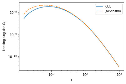
thoughts and ideas as to why this might happen are welcome!

Hi, I was trying to compare the results of my project with the Angular Power Spectrum obtained using Jax-cosmo and CCL, but I've noticed that the two libraries seem to disagree in particular situation. For instance, I've implemented a simple working example as follows:

  cosmo_ccl = ccl.Cosmology(
  Omega_c=0.2589, Omega_b=0.0486, 
  h=0.6774, sigma8 = 0.8159, n_s=0.9667, Neff=0,
  transfer_function='eisenstein_hu', matter_power_spectrum='halofit')
  cosmo_jc = jc.Planck15()
  z_source=1.
  l= np.logspace(2.2,4, 250)
  z = linspace(0,2,2048)
  pz = zeros_like(z)
  pz[argmin(abs(z_source - z))] = 1. 
  nzs_s=jc.redshift.kde_nz(z, pz, bw=0.01)
  tracer=ccl.WeakLensingTracer(cosmo_ccl, (z, nzs_s(z)), use_A_ia=False)
  cl_ccl = ccl.angular_cl(cosmo_ccl, tracer, tracer, l) 
  probes = [ jc.probes.WeakLensing([nzs_s], sigma_e=0.26) ]
  cls = jc.angular_cl.angular_cl(cosmo_jc, l, probes)

and I get the following result:

We suppose that problem is due to the fact that the redshift distribution is a single source plane. @EiffL suggested to add a new type of redshift distribution in this file defined by a single non-null redshift.

Currently we do not include magnification or RSD in the number counts probe. We might want to add those. The formula for these in the the Limber approximation are conveniently summarized in the CCL paper: https://arxiv.org/abs/1812.05995 Sec. 3.3.1

It would have to follow a similar design as for the IA contribution to WL which can be found in jax_cosmo.probes

I'm opening this issue to collect ideas for validation tests and demo.

Thanks to @chihway here are a few options that would progressively demonstrate the code:

• Step 1: A 2 params Fisher + MCMC, for instance on a simple cosmic shear 1 bin example. This builds confidence that everything is going OK
• Step 2: Make the problem more complicated with like sigma8 omegam, and just something that makes Fisher unstable, show that jax-cosmo is still fine compared to chains
• Step 3: A full 3x2pt beyond Fisher, maybe with VI, maybe with Bayes Fast

I guess all of this can be done with cosmosis, it's just a matter of defining the right setup... and checking that the code works against a non-CCL thing.

I'm opening this issue to discuss what the core API regarding cosmology should look like.

Here are several options:

• Cosmologies can be simply dictionaries, that will be passed all the time
• Cosmologies can be full classes kind of what cosmicpy was doing
• Cosmologies can some kind of Module, i.e. keeps all the variable accessible like in a TF Module

But.... I think I want a functional API... not object oriented

Missing np in log, inside Eisenstein-Hu, type=-'eisenhu'.

Discussing with @eelregit here are few ideas of things to improve:

• Allow parameterisation in terms of As
• Allow for flattening of the cosmology object
• Switch to jax.numpy.interp !
• Try to use jax.experimental.odeint instead of jax_cosmo.ode
• Configuration parameters stored in cosmo structure
• include_logdet flag in gaussian_log_likelihood is reversed
• Not sure if transverse_comoving_distance is actually jittable

I think it's important that the code should not only have good performance but also be stilish ^^' As a way to ensure that, I really like the black project. I only have issue with it
it's that it's using 4 space indentation, when I really really like 2 spaces >.<
But Black being the "The Uncompromising Code Formatter" of course they will not compromise on the
indentation......

In any case, I'm opening this issue to see if anyone has thoughts on this, and otherwise I'll try to open a PR to add python code formatting

Hi,
jax.numpy has an interp method since August 2020, with the same API, so I guess we can switch to this JAX implementation instead of https://github.com/DifferentiableUniverseInitiative/jax_cosmo/blob/master/jax_cosmo/scipy/interpolate.py

Currently we only produce angular Cls. we need another integration step to turn these Cls into correlation functions. It's essentially a matter of integration over Bessel functions, it's documented in the CCL paper for example https://arxiv.org/abs/1812.05995 and this method requires an implementation of FFTLog, which can already be found in Python form here: https://github.com/JoeMcEwen/FAST-PT/blob/master/fastpt/HT.py

It's "just" a matter of turning that code to JAX.

It's necessary if we want to fully reproduce smthg like DES Y1, but not a priority as long as we remain at the level demos and forecasts, where things can remain in the angular cls space.

The present halofit code (power.py) does not introduce any fnu correction. Notice that this correction is coded differently in CCL and CLASS. Here is the CLASS comment

     pk_halo = a*pow(y,f1*3.)/(1.+b*pow(y,f2)+pow(f3*c*y,3.-gam));
      pk_halo=pk_halo/(1+xmu*pow(y,-1)+xnu*pow(y,-2))*(1+fnu*0.977);

      /* until v2.9.3 pk_halo did contain an additional correction
         coming from Simeon Bird: the last factor was
         (1+fnu*(0.977-18.015*(pba->Omega0_m-0.3))). It seems that Bird
         gave it up later in his CAMB implementation and thus we also
         removed it. */
      // rk is in 1/Mpc, 47.48and 1.5 in Mpc**-2, so we need an h**2 here (Credits Antonio J. Cuesta)

CCL implements the (1+fnu*(0.977-18.015*(pba->Omega0_m-0.3))) factor.

We only have an EH linear power spectrum currently, and should implement some non-linear corrections.
I have placed in jax_cosmo/nonlinear.py some code inherited from comicpy for smith et al. 2003 non-linear corrections. But I haven't turned it into proper working code yet.

We should:

• Implement a standard mechanism for non-linear corrections in jax_cosmo/power.py
• Add specific utilities for a given correction in jax_cosmo/nonlinear.py

Colab now runs jax v0.2, and apparently some of our code is no longer working. This PR is to track bugs and fixes to update to recent jax version.

Currently, functions like H(cosmo, a), radial_comoving_distance(cosmo, a), etc... which live in background.py are using a functional API. We could instead have these functions be methods of a Cosmology object.

The question is... which interface is better:

chi = bkgr.radial_comoving_distance(cosmo, a)

or

chi = cosmo.radial_comoving_distance(a)

Probably the second one...... But I'm asking just in case some people have some thoughts on this before switching

Should all functions be parameterized by the redshift z or the scale factor a ?

I have heard both sides on this.... I have had a preference myself for a in the past, but I'm getting very annoyed at having to convert between redshift and scale factors all the time....

Could we just parameterize everything in terms of z and call it a day?

First thing to do is to add a base cosmology module, for instance taking inspiration from my old https://github.com/cosmicpy/cosmicpy/blob/master/cosmicpy/cosmology.py

This issue is to track the implementation of a lensing tracer.

The "problem" is that the previous implementations I have all compute the nested integrals in terms of z or a, but we can't evaluate easily a_of_chi(chi), only chi_of_a(a) so I just want to double check here that I'm getting the math correctly for the expression of the intergrals in terms of a.

In any case, what we want to implement here is:

• something that can grab an nz, probably as a function
• compute the lensing efficiency kernel over the nz
• return a kernel function, for further use by the angular CL module

Hello guys,

Starting to use jax_cosmo and I have warnings concerning the current (pip) implementations

Users/rigault/miniforge3/lib/python3.9/site-packages/jax_cosmo/scipy/interpolate.py:35: UserWarning: Explicitly requested dtype <class 'jax.numpy.int64'> requested in astype is not available, and will be truncated to dtype int32. To enable more dtypes, set the jax_enable_x64 configuration option or the JAX_ENABLE_X64 shell environment variable. See https://github.com/google/jax#current-gotchas for more.
s = np.sign(np.clip(x, xp[1], xp[-2]) - xi).astype(np.int64)
/Users/rigault/miniforge3/lib/python3.9/site-packages/jax_cosmo/scipy/interpolate.py:36: UserWarning: Explicitly requested dtype <class 'jax.numpy.int64'> requested in astype is not available, and will be truncated to dtype int32. To enable more dtypes, set the jax_enable_x64 configuration option or the JAX_ENABLE_X64 shell environment variable. See https://github.com/google/jax#current-gotchas for more.
a = (fp[ind + np.copysign(1, s).astype(np.int64)] - fp[ind]) / (
/Users/rigault/miniforge3/lib/python3.9/site-packages/jax_cosmo/scipy/interpolate.py:37: UserWarning: Explicitly requested dtype <class 'jax.numpy.int64'> requested in astype is not available, and will be truncated to dtype int32. To enable more dtypes, set the jax_enable_x64 configuration option or the JAX_ENABLE_X64 shell environment variable. See https://github.com/google/jax#current-gotchas for more.
xp[ind + np.copysign(1, s).astype(np.int64)] - xp[ind]

It is likely connected to the jax version.

I am running with jax v0.4.1

Hey folks, I just came across the repository and wanted to highlight a use-case. Getting JAX up and running with the proper CUDA and CUDNN versions can be a hassle and IMO Docker is the quickest workaround for easy onboarding and setup. It'd be much easier if there was a Dockerfile provided or even an Image on Docker-hub or the Github Container Registry (ghcr.io). That would make reproducibility and benchmarking much easier. At the moment, JAX is a bit spotty with their Docker configurations, but the tensorflow-gpu image works perfectly as a base and already contains many of the needed packages. Having a Dockerfile could also help in creating and writing slightly compute heavy examples with proper accelerator (GPU/TPU) setup.

For now, we have various configuration options distributed everywhere in the code, the idea being
that with a functional API, you can just specify the parameter to the function doing the computation. The problem is that some quantities are being used in multiple places internally by other functions, so we need to make sure that the same options are being used consistently, storing these options in the cosmology seems to make the most sense.

For instance, the choice of transfer function or non-linear prescription currently requires us to carry a specfic function in all functions that need to compute a power spectrum, but this could simply be a flag in the cosmology object. So, let's do that.

I think we want to follow the same approach as in CCL, i.e. we define tracers for all sorts of observables, each tracer allows for the computation of a kernel, and the angular cl code just grabs a list of tracers, power spectrum prescription, and computes the CLs.

So, the angular cl API could look like:

>>> tracer1 = WeakLensingTracer(nz, IA='none')
>>> tracer2 = WeakLensingTracer(nz, IA='none')
>>> cl = angular_cl(cosmo, ell, tracer_1, tracer_2, matter_power_fn)

:-/ or if we go full functional, could look like this:

>>> kernel1 = get_lensing_kernel(nz, IA='none')
>>> kernel2 = get_lensing_kernel(nz, IA='none')
>>> angular_cl = get_angular_cl(cosmo, kernel_fn1=kernel1, kernel_fn2=kernel2, matter_power_fn)
>>> angular_cl(ell)

Hummm.... Thoughts and ideas welcome

I am running docs/notebooks/jax-cosmo-intro on colab with a CPU-only runtime and the following line:

F = - hessian_loglik(params)

gives a mysterious error:

TypeError: Integers cannot be raised to negative powers, got integer_pow(ShapedArray(int32[513,1]), -2)

Any idea why this is being traced with an integer array here?

So, after a few tests, batching with jax.vmap works really great :-) It's pretty magical actually!

So for instance:

def loss(om):
    cosmo = jc.Planck15(Omega_c=om)
    k = np.logspace(-2,1)
    return np.sum(jc.power.linear_matter_power(cosmo, k)**2)

grads = jax.jit(jax.grad(loss))
%timeit grads(0.3).block_until_ready()

clocks in at 129ms, which ok, should probably be faster, but ok.

And now if you do:

batched_grads = jax.jit(jax.vmap(grads))
%timeit batched_grads(np.ones(32)*0.3).block_until_ready()

I get the same 129 ms \o/, despite now computing the pk for a batch of 32 cosmologies :-D And my GPU doesn't go above 30% usage.

Now the problem is that if I try to do something similar at the level of the observed
Cls, it doesn't work, I can't make more than like one batch, and it's because of the nested intergrations, that currently work by vectorizing the evalutation of the integrands. So at some point in the graph if you have 2 integrals that require each 512 points, you already have 512x512x....xBatch dimensions arrays.

So I think we need to replace simps. by a sequential version of that, with an integration loop instead of just batched evaluation of a function. The integral itself may end up being slower, but will have a hugely reduced memory footprint.

Right now we let JAX fgure out the gradients automatically for integration, that works ok but I think it's causing large memory overhead, and when autodiffing lax.scan calls the graph takes very long to compile. So instead, we probably should implement custom JVP for integrals. Which is easy, it's just the integral of the inner JVP.

I'm openning this issue to document my experimentations with this and gather any thoughts or ideas anyone may have.

To get things started, here is my first attempt at a custom Simpson integration using jax.lax scan and custom JVP:

def my_simps(func, a,b, *args, N=128):
    if N % 2 == 1:
        raise ValueError("N must be an even integer.")
    dx = (b-a)/N
    x = np.linspace(a,b,N+1)
    return _custom_simps(func, x, dx, *args)

@partial(custom_jvp, nondiff_argnums=(0,1,2))
def _custom_simps(func, x, dx, *args):
    f = lambda x: func(x, *args)
    @jax.remat
    def loop_fn(carry, x):
        y = f(x)
        s = 4*y[0] + 2*y[1]
        return carry+s, 0
    r, _ = jax.lax.scan(loop_fn, f(np.atleast_1d(x[0]))[0], x[1:].reshape((-1,2)))
    S = dx/3 * ( r - f(np.atleast_1d(x[-1]))[0])
    return S

@_custom_simps.defjvp
def _custom_simps_jvp(func, x, dx, primals, tangents):
    # Define a new function that computes the jvp
    f = lambda x: jax.jvp(lambda *args:func(x, *args), primals, tangents)

    def loop_fn(carry, x):
        c, *args=carry
        s1 = f(x[0])
        s2 = f(x[1])
        return jax.tree_multimap(lambda a,b,c:a+4*b+2*c, carry, s1,s2), 0

    r, _ = jax.lax.scan(loop_fn, f(x[0]), x[1:].reshape((-1,2)))
    S = jax.tree_multimap(lambda a,b: dx/3 * (a-b), r, f(x[-1]))
    return S

It seems to work in simple examples, but is still hitting a strange issue in the lax.scan_tranpose function used in reverse mode AD

it'd be great to implement a couple of functions to compute a mu(z) calculation (e.g. for supernova cosmology).

I've whipped up a couple of functions that work on my end within a Numpyro-based BHM sampler (based on BAHAMAS)

import jax.numpy as np
from jax import grad, jit, vmap, random, lax
import jax
import jax_cosmo as jc
import scipy.constants as cnst

inference_type = "w"

# the integrand in the calculation of mu from z,cosmology
@jit
def integrand(zba, omegam, omegade, w):
    return 1.0/np.sqrt(
        omegam*(1+zba)**3 + omegade*(1+zba)**(3.+3.*w) + (1.-omegam-omegade)*(1.+zba)**2
    )

# integration of the integrand given above, vmapped over z-axis
@jit
def hubble(z,omegam, omegade,w):
    # method for calculating the integral
    fn = lambda z: jc.scipy.integrate.romb(integrand,0., z, args=(omegam,omegade,w)) #[0]
    I = jax.vmap(fn)(z)
    return I

then we can compute a Dlz that changes with the curvature value omegakmag by defining a couple of lax conditional statements

@jit
def Dlz(omegam, omegade, h, z, w, z_helio):

    # which inference are we doing ?
    if inference_type == "omegade":
      omegakmag =  np.sqrt(np.abs(1-omegam-omegade))  
    else:
      omegakmag = 0.

    hubbleint = hubble(z,omegam,omegade,w)
    condition1 = (omegam + omegade == 1) # return True if = 1 
    condition2 = (omegam + omegade > 1.)

    #if (omegam+omegade)>1:
    def ifbigger(omegakmag):
      return (cnst.c*1e-5 *(1+z_helio)/(h*omegakmag)) * np.sin(hubbleint*omegakmag)

    # if (omegam+omegade)<1:
    def ifsmaller(omegakmag):
      return cnst.c*1e-5 *(1+z_helio)/(h*omegakmag) *np.sinh(hubbleint*omegakmag)   

    # if (omegam+omegade==1):
    def equalfun(omegakmag):
      return cnst.c*1e-5 *(1+z_helio)* hubbleint/h

    # if not equal, default to >1 condition
    def notequalfun(omegakmag):
      return lax.cond(condition2, true_fun=ifbigger, false_fun=ifsmaller, operand=omegakmag)

    distance = lax.cond(condition1, true_fun=equalfun, false_fun=notequalfun, operand=omegakmag)

    return distance


# muz: distance modulus as function of params, redshift
@jit
def muz(omegam, w, z):
    z_helio = z # should this be different ?
    omegade = 1. - omegam
    #w = -1.0 # freeze w
    h = 0.72
    return (5.0 * np.log10(Dlz(omegam, omegade, h, z, w, z_helio))+25.)

the calculation for 500 supernova distances is super quick:

zs = np.linspace(0, 1.2, num=500)
print('time to compute 500 SNIa distance integrals:')
%time mymus = muz(0.3, 0.7, zs)
plt.plot(zs, mymus, label='fid')

plt.xlabel(r'$z$')
plt.ylabel(r'$\mu(z; \mathcal{C})$')
plt.legend()
plt.show()

time to compute 500 SNIa distance integrals:
CPU times: user 1.23 s, sys: 9.98 ms, total: 1.24 s
Wall time: 1.28 s

A lot of this might be redundant, but would be great to see integrated into the full package. I'm polishing my sampler code on my end, so at the very least these functions could live over there.

Hi!
I am reproducing the tutorial for counts clustering.

Requesting covariance matrix in full shape (sparse = False)
mu, cov = jc.angular_cl.gaussian_cl_covariance_and_mean(cosmo, ell, probes, sparse=False)

returns error
TypeError: _transpose() got an unexpected keyword argument 'axes'
with this line from angular_cl.py:
cov_mat = cov_mat.transpose(axes=(0, 2, 1, 3)).(n_ell * n_cls, n_ell * n_cls))

I changed the source line code to
cov_mat = np.transpose(cov_mat, axes=(0, 2, 1, 3)).(n_ell * n_cls, n_ell * n_cls))
and the error disappeared. I don't know, probably it is related to newer versions of jax.numpy.

The returned non-sparse matrix equals to jc.sparse.to_dense(cov_sparse).

Package versions are:

JAX version: 0.2.18
jax-cosmo version: 0.1rc7

By the way:
I running the tutorial and the Cls calculations by jax cosmo is ~40 sec in opposition to CCL's 0.2 sec for 1x1, 1x2 and 2x2 cross correlations. What I am doing wrong?

Thanks.

This issue makes the current tests fail on CI.

It corresponds to the specific test in test_sparse.py :

X = np.array(
    [
        [[1, 2, 3], [4, 5, 6], [-1, 7, -2]],
        [[1, 2, 3], [-4, -5, -6], [2, -3, 9]],
        [[7, 8, 9], [5, -4, 6], [-3, -2, -1]],
    ]
)
assert_array_equal(det(0.0 * X), 0.0)

I traced it back to the second call of _block_det() in the for-loop of slogdet() : and can therefore be reproduced with

sparse = 0.0 * X
i = 1
N = 3
P = 3
print(_block_det(sparse, i, N, P))

Ping @dkirkby

JAX doesn't have yet all of the scipy interpolation tools, so we need our own.

Currently we only have a trivial linear interpolant here:

But would be great higher precision interpolation methods, this reduces the cost/size of interpolation tables for a given accuracy, and that is the main limiting factor in the growth or comoving distance calculation right now.

A spline interpolation method similar to
https://docs.scipy.org/doc/scipy-0.18.1/reference/generated/scipy.interpolate.UnivariateSpline.html#scipy.interpolate.UnivariateSpline

here is a list of 10 pathological sets of cosmo parameters that make the Cl WL NaN
The use-cas is the DESY_Y1_shear exercice

m1,m2,m3,m4,dz1,dz2,dz3,dz4 = [0.]*8
A,eta = [1.]*2


data = np.array([[ 0.24986424,  0.55773633,  0.04630792,  0.61299905,  0.99486902,
        -1.44603776],
       [ 0.17611082,  0.71919114,  0.05874876,  0.67659724,  0.95329858,
        -1.41323164],
       [ 0.11939933,  0.44445573,  0.06162388,  0.79803975,  1.00682757,
        -1.77138837],
       [ 0.21723086,  0.4209687 ,  0.03940861,  0.73820567,  1.05830809,
        -1.77511559],
       [ 0.45726321,  0.60605765,  0.05444171,  0.62133009,  0.88678424,
        -1.83988558],
       [ 0.11030471,  0.49406485,  0.05778253,  0.88668811,  0.97388076,
        -1.94438598],
       [ 0.23417783,  0.6072679 ,  0.03107563,  0.72839096,  0.91472034,
        -0.94570266],
       [ 0.31449189,  0.48404425,  0.05613155,  0.56604649,  0.91932335,
        -1.11252456],
       [ 0.42029479,  0.40920462,  0.03177297,  0.76163707,  0.93350105,
        -1.78184122],
       [ 0.35075444,  0.43376266,  0.03103901,  0.65861007,  0.99913718,
        -1.70636958]])

# example
Omega_c,sigma8,Omega_b,h,n_s,w0 = data[0]

cosmo = FiducialCosmo(Omega_c=Omega_c, sigma8=sigma8, Omega_b=Omega_b,
                          h=h, n_s=n_s, w0=w0)
debug_model_fn(get_params_vec(cosmo, [m1, m2,m3, m4], [dz1, dz2, dz3, dz4], [A, eta]))

After a little bit of digging, it would technically be possible to fully wrap either code in jax-cosmo, using finite difference to get an approximation of gradients. Just for future reference, or if someone wants to do it, here is the procedure:

• The easy part, adding a new JAX primitive, essentially, just telling JAX how to manipulate your function, see here: https://jax.readthedocs.io/en/latest/notebooks/How_JAX_primitives_work.html#Defining-new-JAX-primitives . You can define a custom JVP based on finite differences, so that you can get approximate gradients within the rest of the computation.

• The not so easy part: Adding an XLA custom op to perform the computation. So the problem is that doing the above will work, but you can't JIT your program. For that, you would need to define a custom XLA op in C++ that would call CLASS/CAMB. It's technically possible, but painful >.< .... Here is the XLA reference for custom CPU ops: https://www.tensorflow.org/xla/custom_call

• Another option that is probably easier than the previous one, there is an experimental API for host callbacks in Pythton: https://github.com/google/jax/blob/master/jax/experimental/host_callback.py
  With that, we should be able to have CLASS and CAMB interfaces just from the python, and it actually gets wrapped around in the XLA compiled code :-D

Hi,
if you use in jax_cosmo/notebooks/CCL_comparison.ipynb

# We first define equivalent CCL and jax_cosmo cosmologies

Omega_c_fidu =  0.2589
sigma8_fidu  = 0.8159
Omega_b_fidu = 0.0486 
h_fidu       = 0.6774 
n_s_fidu     =  0.9667 
w0_fidu      = -1.0

params_fidu = [Omega_c_fidu,sigma8_fidu,Omega_b_fidu,h_fidu,n_s_fidu,w0_fidu]


params_pathos =[[ 0.24986424,  0.55773633,  0.04630792,  0.61299905,  0.99486902,
        -1.44603776],
       [ 0.17611082,  0.71919114,  0.05874876,  0.67659724,  0.95329858,
        -1.41323164],
       [ 0.11939933,  0.44445573,  0.06162388,  0.79803975,  1.00682757,
        -1.77138837],
       [ 0.21723086,  0.4209687 ,  0.03940861,  0.73820567,  1.05830809,
        -1.77511559],
       [ 0.45726321,  0.60605765,  0.05444171,  0.62133009,  0.88678424,
        -1.83988558],
       [ 0.11030471,  0.49406485,  0.05778253,  0.88668811,  0.97388076,
        -1.94438598],
       [ 0.23417783,  0.6072679 ,  0.03107563,  0.72839096,  0.91472034,
        -0.94570266],
       [ 0.31449189,  0.48404425,  0.05613155,  0.56604649,  0.91932335,
        -1.11252456],
       [ 0.42029479,  0.40920462,  0.03177297,  0.76163707,  0.93350105,
        -1.78184122],
       [ 0.35075444,  0.43376266,  0.03103901,  0.65861007,  0.99913718,
        -1.70636958]]

params = params_fidu  # Ok

params = params_pathos[0]


Omega_c,sigma8,Omega_b,h,n_s,w0 = params

cosmo_ccl = ccl.Cosmology(
    Omega_c=Omega_c, Omega_b=Omega_b, h=h, sigma8 = sigma8, n_s=n_s, Neff=0,
    transfer_function='eisenstein_hu', matter_power_spectrum='halofit')

cosmo_jax = Cosmology(Omega_c=Omega_c, Omega_b=Omega_b, h=h, sigma8=sigma8, n_s=n_s,
                      Omega_k=0., w0=w0, wa=0.)

There are differences in many places and NaN for Cl in all tests (WL, gg clustering, cross)

In the nb dealing with CCL comparison, here is the code that defines the CCL Cosmology

cosmo_ccl = ccl.Cosmology(
    Omega_c=0.3, Omega_b=0.05, h=0.7, sigma8 = 0.8, n_s=0.96, **Neff=0**,
    transfer_function='eisenstein_hu', matter_power_spectrum='halofit')

Even if in the context of this nb, Neff=0 does not matter, it leads to nasty results in others.
In fact, do not add this parameter and everything is in order.

cosmo_ccl = ccl.Cosmology(
   Omega_c=0.3, Omega_b=0.05, h=0.7, sigma8 = 0.8, n_s=0.96, 
   transfer_function='eisenstein_hu', matter_power_spectrum='halofit')

We need a power spectrum, I'm thinking using the fitting formula from Eisenstein & Hu 98 is probably going to provide good enough results as a first step.

Python code for that can be found here: https://github.com/cosmicpy/cosmicpy/blob/e8636300c62f18f115601c59a05b96ce2b427ea2/cosmicpy/cosmology.py#L584

Hi,
concerning radial_comoving_distance at low z (< 5e-2)

def radial_comoving_distance(cosmo, a, log10_amin=-3, steps=256)

the number of steps needs to be increased to 1024.

If one sets

cosmo_jax = Cosmology(
    Omega_c=0.2545,
    Omega_b=0.0485,
    h=0.682,
    Omega_k=0.0,
    w0=-1.0,
    wa=0.0  
###  other params if needed
)
z = jnp.logspace(-3, 3,100)
grad_lum = vmap(grad(luminosity_distance), in_axes=(None,0))(cosmo_jax,z2a(z))

# direct integration d(d_L)/dOmega_k(cosmo_jax)
func = lambda a: -0.5*const.rh * (-1.+1./a**2) / (a**2 * Esqr(cosmo_jax, a)**1.5)
dLdOmega_k = quadIntegral(func,z2a(z),1.0,ClenshawCurtisQuad(100))*(1+z) 

plt.figure(figsize=(10,10))
plt.plot(z,grad_lum.Omega_c/cosmo_jax.h,ls='-',lw=3,label=r"$\frac{\partial d_L}{\partial \Omega_c}$")
plt.plot(z,grad_lum.Omega_b/cosmo_jax.h,ls='--',lw=3, label=r"$\frac{\partial d_L}{\partial \Omega_b}$")
plt.plot(z,grad_lum.h/cosmo_jax.h,ls='--',lw=3, label=r"$\frac{\partial d_L}{\partial h}$")
plt.plot(z,grad_lum.Omega_k/cosmo_jax.h,ls='-',lw=3, label=r"$\frac{\partial d_L}{\partial \Omega_k}$")
plt.plot(z,grad_lum.w0/cosmo_jax.h,ls='--',lw=3, label=r"$\frac{\partial d_L}{\partial w_0}$")
plt.plot(z,grad_lum.wa/cosmo_jax.h,ls='--',lw=3, label=r"$\frac{\partial d_L}{\partial w_a}$")
plt.plot(z,dLdOmega_k/cosmo_jax.h, ls='--',lw=3,c='k',label=r"Direct Integ: $\frac{\partial d_L}{\partial \Omega_k}$")
plt.yscale("symlog")
plt.xscale("log")
plt.legend()
plt.grid();

leads to a perfect matching (black vs red curves)

While using 256 steps leads to a discrepancy (black vs red curves):

The time has come to follow the all-contributors guidelines. I'm opening this issue to add people that have already contributed.

Finally, we need to implement the integration over window functions and Pk. Unfortunately Jax doesnt implement yet any complicated integration procedure, so we will probably have to resort to some Simpson rule or something.

To be able to replicate a simple DES Y1 or LSST SRD analysis we need an IA model, we'll go ahead and implement the NLA.