devinterview-io / logistic-regression-interview-questions

🟣 Logistic Regression interview questions and answers to help you prepare for your next machine learning and data science interview in 2024.

50 Core Logistic Regression Interview Questions

You can also find all 50 answers here 👉 Devinterview.io - Logistic Regression

1. What is logistic regression and how does it differ from linear regression?

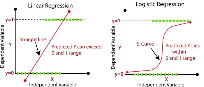
Logistic Regression is designed to deal with binary classification tasks. Unlike Linear Regression, it doesn’t use a direct linear mapping for classification but rather employs a sigmoid function, offering results in the range of 0 to 1.

Sigmoid Function

The sigmoid function is integral to logistic regression. It maps continuous input values (commonly called a linear combination of weights and features, or logits) to a probability range (0 to 1).

The sigmoid function, often denoted by $\sigma(z)$, is expressed as:

$$ \sigma(z) = \frac{1}{1 + e^{-z}} $$

where $z$ represents the linear combination:

$$ z = w_0x_0 + w_1x_1 + ... + w_nx_n $$

• $x_n$ are the input features,
• $w_n$ are the co-efficients
• $w_0$ is the bias term.

Decision Boundary

Logistic Regression fits a decision boundary through the dataset. Data points are then classified based on which side they fall.

Using the sigmoid function, if $\sigma(z)$ is greater than 0.5, the predicted class is 1. Otherwise, it's 0.

Probability & Thresholding

Logistic Regression provides a probability score for each class assignment. You can then use a threshold to declare the final class; a common threshold is 0.5.

Loss Functions

While linear regression uses the mean squared error (MSE) or mean absolute error (MAE) for optimization, logistic regression employs the logarithmic loss, also known as the binary cross-entropy loss:

$$ \text{BCE}(y, \hat{y}) = -y\log(\hat{y}) - (1-y)\log(1-\hat{y}) $$

where:

• $y$ is the actual class (0 or 1)
• $\hat{y}$ is the predicted probability by the model.

Complexity and Training

Logistic Regression involves the iteration of minimization techniques like gradient descent. This training often converges faster than linear regression's training process.

Regularization

Both linear and logistic regressions can integrate regularization techniques (e.g. L1, L2) to avoid overfitting. If needed, the emphasis can be shifted from minimizing the loss function to regulating the coefficients, ultimately enhancing model generalization.

2. Can you explain the concept of the logit function in logistic regression?

The Logit function is a crucial component of Logistic Regression, serving as the link function that connects a continuous input space to a binary output space.

The Role of the Logit Function

• Input: A continuous range from $-\infty, \infty$.
• Output: A probability score bounded in $(0, 1)$.

The log-odds transformation ensures that the output falls within a valid probability range.

Mathematical Representation

The logit function is defined as:

$$ \text{logit}(p) = \ln\left(\frac{p}{1-p}\right) $$

where $p$ typically represents the probability of an event occurring. After applying the sigmoid function to the logit output, it becomes:

$$ \sigma(z) = \frac{1}{1 + e^{-z}} $$

where $z$ denotes the log-odds ratio calculated using the logit function:

$$ z = \text{logit}(p) = \ln\left(\frac{p}{1-p}\right) $$

Visual Representation

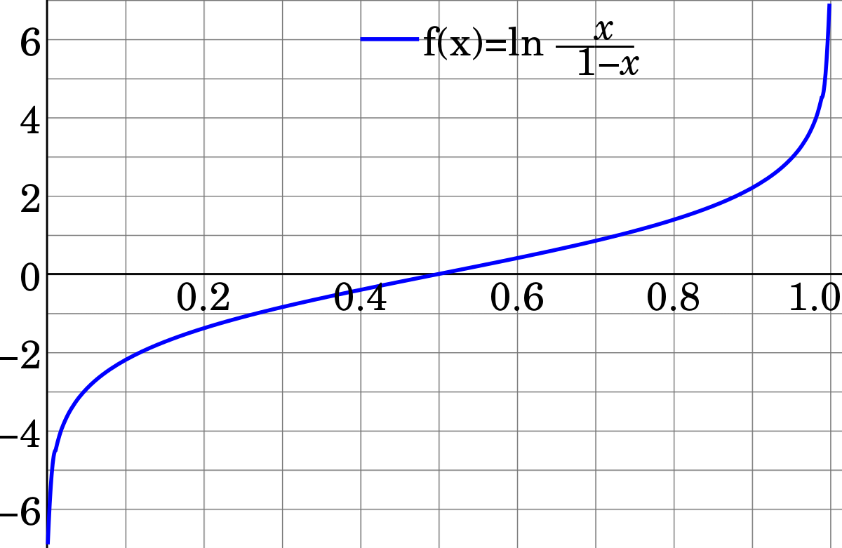
The logit function maps a probability estimate onto a continuous range which can then be transformed into a binary outcome via the decision boundary $\theta$.

Code Example: Logit Transformation

Here is the Python code:

import numpy as np
import matplotlib.pyplot as plt

# Define the logit function
def logit(p):
    return np.log(p / (1 - p))

# Generate linearly spaced probabilities
p_values = np.linspace(0.01, 0.99, 100)
logit_values = logit(p_values)

# Visualize the logit transformation
plt.figure(figsize=(8, 6))
plt.plot(p_values, logit_values, label='Logit Transformation')
plt.axhline(y=0, color='black', linestyle='--', linewidth=0.8)
plt.axvline(x=0.5, color='red', linestyle='--', linewidth=0.8, label='Decision Boundary at 0.5')
plt.xlabel('Probability (p)')
plt.ylabel('Log-Odds Ratio (z)')
plt.title('Logit Transformation')
plt.legend()
plt.grid(True)
plt.show()

3. How is logistic regression used for classification tasks?

Logistic regression remains a powerful tool for binary classification tasks. Despite its name, it's a classification algorithm that models the probability of class membership.

The model achieves this by evaluating the log-odds of the likelihood of an observation belonging to a specific class.

Logistic regression outputs probabilities ranging from 0 to 1 and predicts class membership depending on whether the probability is above or below a threshold, typically taken as 0.5.

Key Concepts

• Sigmoid Function: It transforms any real-valued number to the range (0, 1), signifying the probability of occurring.

$$ \sigma(z) = \frac{1}{1 + e^{-z}} $$ or in the more familiar format, $$ P(Y=1|X) = \frac{1}{1+e^{-(b_0 + b_1X_1 + .... + b_kX_k)}} $$

• Odds Ratio: The probability of success (event) over the probability of failure (non-event).

$$ Odds = \frac{P(Y=1|X)}{1 - P(Y=1|X)} $$

• Log-Odds or Logit Function: It's the natural logarithm of the odds ratio, bringing the range of probabilities from (0, 1) to $(-\infty, \infty)$.

$$ Logit(P(Y=1|X)) = ln\left(\frac{P(Y=1|X)}{1 - P(Y=1|X)}\right) $$

Evaluating Probability

• Threshold Selection: The traditional cutoff is at 0.5, but it can be adjusted, depending on the task. A lower threshold is usually associated with increased sensitivity and reduced specificity.
• Receiver Operating Characteristic (ROC) Curve: It measures the model's ability to differentiate between classes. The area under the curve ($AUC$) is a common performance metric.
• Precision-Recall Curve: Especially useful when there is class imbalance.

Dealing With Multiclass Situations

While logistic regression inherently pertains to binary classification, strategies can be employed to handle multiclass problems:

• One-vs-Rest (OvR), which trains a dedicated model for each class. During prediction, the class with the highest probability output from any classifier is picked.
• One-vs-One (OvO), which constructs models for all possible class pairs, leading to greater computational complexity. The choice is made based on a "voting" mechanism.

Modern software tools, however, often implement these strategies automatically without explicit guidance from the user, making them more straightforward to use.

4. What is the sigmoid function and why is it important in logistic regression?

The sigmoid function (also known as the logistic function) is a crucial element in logistic regression as it maps real-valued numbers to a range between $0$ and $1$.

Mathematical Representation

The sigmoid function is defined as:

$$ \sigma(z) = \frac{1}{1 + e^{-z}} $$

Where:

• $z$ is the input to the function, typically a linear combination of features and weights: $z = w^T x + b$.
• $\sigma(z)$ represents the predicted probability that the output is $1\ (or "positive")$, given the input $x$ parameterized by $w$ and $b$.

Visual Representation

The sigmoid function is S-shaped, transitioning from $0$ to $1$, and it's symmetric around the origin:

$$ $$ \lim_{z \to -\infty} \sigma(z) &= 0 \\ \lim_{z \to \infty} \sigma(z) &= 1 \\ \sigma(0) &= 0.5 $$ $$

Role in Logistic Regression

The key reason for using the sigmoid function in logistic regression is its ability to convert the output of a linear equation (the "log-odds") into a probability.

The probability (

) that a data sample (

) belongs to the positive class (commonly indicated as "1") is given by:

,

where

is the log-odds defined as:

Decision Boundary

The sigmoid function helps define a decision boundary. For any input data point above the boundary, the predicted probability is closer to $1$, and for points below the boundary, the predicted probability is closer to $0$.

The boundary itself is where $\sigma(z) = 0.5$, which corresponds to:

$$ z = w^T x + b $$

and

$$ w^T x + b = 0 $$

Mathematically, this is a hyperplane (for multi-dimensional cases) that separates the two classes, and the sign of $w^T x + b$ reflects the class assignment.

Key Takeaways

• The sigmoid function is essential in logistic regression for probabilistic predictions which are advantageous in classifications.
• It characterizes the nature of a binary decision based on a probability threshold (usually $0.5$).
• The choice of threshold directly influences sensitivity (true positive rate) and specificity (true negative rate), crucial in various real-world applications such as medicine or law enforcement.

Code Example: Sigmoid Function

Here is the Python code:

import numpy as np

# Sigmoid function
def sigmoid(z):
    return 1 / (1 + np.exp(-z))

# Visualize the function
import matplotlib.pyplot as plt

z = np.linspace(-7, 7, 200)
y = sigmoid(z)

plt.plot(z, y)
plt.xlabel('z')
plt.ylabel('σ(z)')
plt.title('Sigmoid Function')
plt.grid(True)
plt.show()

5. Discuss the probability interpretations of logistic regression outputs.

Logistic Regression outputs probabilities by using a logistic function, represented by:

$$ \sigma(z) = \frac{1}{1 + e^{-z}} $$

Where $z$ is the linear combination of input features and their corresponding coefficients:

$$ z = w_0x_0 + w_1x_1 + \ldots + w_nx_n $$

The probabilities $\sigma(z)$ are then used to make binary classification decisions.

6. What are the assumptions made by logistic regression models?

Logistic Regression makes several key assumptions about the data in order to produce reliable results.

Assumptions of Logistic Regression

1. Binary or Ordinal Outcomes: Logistic Regression is ideal for predicting binary outcomes, but when used with multiple categories, the model assumes that these categories are ordered.

2. Independence of Observations: Each data point should be independent of others.

3. Absence of Multicollinearity: There should be minimal correlation among independent variables. The presence of high multicollinearity can make interpretation of the model difficult.

4. Linearity of Independent Variables and Log Odds: The relationship between predictors and the log-odds of the outcome is assumed to be linear.

5. Significance of Predictors: While the model does not strictly require variable significance, this is often an important practical consideration for model interpretability.

6. Large Sample Sizes: Though often not strictly enforced, logistic regression performs better with larger sample sizes. A general rule of thumb is having at least 10 rare events for each predictor variable.

Validating Assumptions

Researchers use several methods to assess the validity of these assumptions, including hypothesis testing for coefficients, variable-to-variable checks for multicollinearity, and the Hosmer-Lemeshow goodness-of-fit test.

These checks help ensure the stability and reliability of logistic regression models.

For data that deviates significantly from these assumptions, alternative models like Probit or Complementary Log-Log regression can be considered.

7. How does logistic regression perform feature selection?

Logistic regression naturally implements feature selection through mechanisms like L1 regularization (LASSO) which introduce sparsity.

L1 Regularization: Encouraging Sparsity

L1 regularization adds a term to the loss function that is the absolute value of the coefficients. This tends to "shrink" coefficients to zero, effectively removing the associated features. Regularization strength is typically controlled by the parameter $\lambda$.

Mathematically, L1 regularization is expressed as:

Where:

• $\lambda$ determines the strength of regularization, and
• $p$ represents the number of features.

Pros and Cons of L1 Regularization

• Pros: Efficient for high-dimensional datasets and naturally performs feature selection.
• Cons: May lead to instability in feature selection when features are correlated; tends to select only one feature from a group of correlated features.

8. Explain the concept of odds and odds ratio in the context of logistic regression.

In the context of logistic regression and binary classification, the concept of odds is fundamental in understanding the likelihood of an event occurring.

Understanding Odds

• Odds of a positive event: The ratio of the probability that the event happens to the probability that it does not happen: $\frac{P(y=1)}{1 - P(y=1)}$.
• Odds for a negative event: Corresponds to the reciprocal of the odds for a positive event: $\frac{1 - P(y=1)}{P(y=1)}$.

For balanced data with an equal proportion of positive and negative instances, the odds simply reduce to 1.

Understanding Odds Ratio

Odds ratio provides insights into the likelihood of an event occurring under different conditions or scenarios. In the context of logistic regression, it characterizes how the odds of an event are affected by a one-unit change in a predictor variable.

Consider a simple logistic regression with a single predictor variable (feature):

$$ \text{Logit}(\text{odds}) = \beta_0 + \beta_1x $$

The exponential of the coefficient for the predictor variable gives the odds ratio. For instance, if $\beta_1 = 0.7$, then the odds ratio is $e^{0.7} \approx 2.01$. This means that for a one-unit change in the predictor variable, the odds of the positive event (class 1) increase by a factor of approximately 2.01.

In a multivariate logistic regression:

$$ \text{Logit}(\text{odds}) = \beta_0 + \beta_1x_1 + \beta_2x_2 + \ldots + \beta_kx_k $$

each coefficient has its own odds ratio, indicating the multiplicative effect on the odds of the event.

Practical Interpretation

• For a positive event (e.g., "click" in online advertising), an odds ratio greater than 1 indicates a feature that positively influences the occurrence of the event.
• For a negative event (e.g., "churn" in customer retention), an odds ratio less than 1 indicates a feature associated with lower odds of the event occurring.

Typically, understanding the odds and odds ratio is crucial for interpreting model outputs and identifying the most influential predictors.

9. How do you interpret the coefficients of a logistic regression model?

Logistic Regression is popular for binary classification due to its interpretability. By analyzing the model's coefficients, we can deduce the influence of input features on the output class.

Understanding Coefficients

In a Logistic Regression model, the log-odds of an event occurring are expressed as a linear combination of features with weights or coefficients. This is represented as:

$$ \log\left(\frac{{P(Y=1)}}{{1-P(Y=1)}}\right) = \beta_0 + \beta_1x_1 + \ldots + \beta_kx_k $$

where:

• $\beta_0, \ldots, \beta_k$ are the coefficients.
• $x_1, \ldots, x_k$ are the features.
• $P(Y=1)$ is the probability of the positive class.

Using the logistic function $f(z) = \frac{1}{1 + e^{-z}}$, the relationship between the log-odds and the probability of the positive class $P(Y=1)$ is established.

Interpreting Coefficients

• Sign: If a coefficient is positive, an increase in the corresponding feature value makes it more likely for the target class to be positive. If it's negative, the likelihood decreases.

• Magnitude: The absolute value of a coefficient relates to its feature's impact on the target class probability. A larger magnitude indicates a stronger influence.

• Odds-Ratio: It's the exponentiated coefficient. An odds-ratio greater than 1 suggests that, for a unit increase in the feature, the odds of the positive class increase. A value less than 1 suggests a decrease in odds.

• Predictive Power: Coefficients are used to generate probability predictions:

$$ P(Y=1) = \frac{1}{{1+e^{-(\beta_0 + \beta_1x_1 + \ldots + \beta_kx_k)}}} $$

• Confidence Interval: A confidence interval for a coefficient provides a range, within which we are confident lies the true value of the coefficient, based on our sample.

10. Describe the maximum likelihood estimation as it applies to logistic regression.

Maximum Likelihood Estimation (MLE) in the context of Logistic Regression aims to find the parameter values that make the observed data most probable.

The MLE Process

1. Define the Likelihood Function: For a binary outcome (0 or 1), MLE seeks the set of parameters $\beta_0, \beta_1, ..., \beta_k$ that maximizes the probability of observing the given outcomes $y_1, y_2, ..., y_n$, assuming a logistic distribution.

2. Transform to Log-Likelihood: The log-likelihood simplifies calculations due to its mathematical properties, such as converting products into sums.

$$ \ell(\beta) = \log L(\beta) $$

3. Determine the Derivative: The derivative of the log-likelihood function helps identify the maximum. Techniques like gradient ascent are used for optimization.

4. Estimate Coefficients: By maximizing the log-likelihood function, we estimate the coefficients $\beta$ that best fit the data.

5. Obtain Standard Errors: Their ratio can provide insights into possible multicollinearity issues.

MLE and Model Accuracy

• Confusion Matrix: MLE could overfit the data, becoming overly sensitive to the training set.
• Accuracy: The approach indirectly maximizes the model's accuracy, focusing on achieving the best parameter set to fit the given data.
• Sensitivity and Specificity: MLE can potentially tune the model to favor one over the other.

11. How do you handle categorical variables in logistic regression?

While it's true that logistic regression is designed for binary outcomes, it's still possible to work with categorical predictors by transforming them into a suitable format for logistic regression. Key strategies include binary encoding, dummy variables, and effect coding.

Encoding Strategies

1. Binary Encoding: Represents each unique category with an increasing binary bit pattern. Although this reduces the number of features, its interpretability can be compromised.

   Example: $A \rightarrow 00, B \rightarrow 01, C \rightarrow 10$

2. Using Dummy Variables: This straightforward approach creates a binary variable for each category. One category is omitted to avoid collinearity, especially when there's a constant term.

3. Effect Coding: Here, categories are coded relative to a reference category, with the reference category typically assigned a fixed effect of -1. This approach is mainly used in ANOVA and can be suitable when the categories are nominal rather than ordinal.

   Example: $A$ is the reference category. So the effect coding would be: $A \rightarrow -1, B \rightarrow 0, C \rightarrow 1$

Best Practices

• Category Size and Log Odds: For smaller datasets, it's essential to ensure that each category has a sufficient representation in the data.
• Overfitting Concerns: When dealing with a large number of categories, especially in the case of high-cardinality variables, there is a risk of overfitting, which might make the model generalized to your dataset.

12. Can logistic regression be used for more than two classes? If so, how?

Yes, multiclass logistic regression, also known as softmax regression, uses a similar concept to the binary logistic regression.

Binary Logistic Regression vs. Multiclass Logistic Regression

• Binary Logistic Regression: Used for binary classification problems, where the output is one of two classes.

  • Activation Function: Utilizes the sigmoid function to map any real-valued number to a value between 0 and 1.
  • Decision Boundary: Results in a single cutoff point that separates the two classes.

• Multiclass Logistic Regression (Softmax Regression): Suitable for problems with three or more mutually exclusive classes (exclusive means that each observation belongs to only one class).

  • Activation Function: Applies the softmax function to assign probabilities to each class, ensuring the sum of probabilities across all classes is 1.
  • Decision Boundary: Does not establish a sharp boundary but instead provides probabilities for each class.

13. Discuss the consequences of multicollinearity in logistic regression.

Multicollinearity in the context of logistic regression refers to the high correlation between predictor variables. This can lead to several issues in the model.

Consequences of Multicollinearity

1. Increased Standard Errors
   High correlation between predictors can lead to unstable parameter estimates. Coefficients may vary considerably across different samples of data. As a result, the standard errors of the coefficient estimates can inflate, making the estimates less reliable.

2. Uninterpretable Coefficients
   Multicollinearity can cause coefficient estimates to be erratic and change in both sign and magnitude with small changes in the model. This erratic behavior makes it difficult to accurately interpret the role of individual predictors in the model.

3. Inconsistent Predictor Importance
   When multicollinearity is present, the importance of the correlated predictors can be difficult to discern. For example, if two variables are highly correlated and one is removed from the model, the effect of the other variable can significantly change.

4. Reduced Statistical Power
   Multicollinearity can make it difficult for logistic regression to identify true relationships between predictors and the outcome variable. This reduced statistical power can lead the model to miss crucial associations between variables.

5. Inaccurate Predictions
   The presence of multicollinearity can lead to inaccurate predictions. When using the logistic regression model to predict outcomes for new data, the uncertainty introduced due to multicollinearity can result in less reliable predictions.

6. Misleading Insights
   Multicollinearity can provide misleading insights about the relationship between the predictors and the outcome variable. This can affect the model's applicability in real-world scenarios, potentially leading to costly or erroneous decisions.

7. Data-Specific Findings
   Multicollinearity can result in model findings that are specific to the dataset used, limiting the model's generalizability to other datasets or populations.

Identifying and Dealing with Multicollinearity

Identifying Multicollinearity

1. Correlation Matrix: Identify pairs of predictors with high correlation.
2. VIF (Variance Inflation Factor): VIF quantifies the severity of multicollinearity in the regression model. Generally, VIF values above 5 or 10 are considered as indicating multicollinearity.

Dealing with Multicollinearity

1. Variable Selection:

   • Use domain knowledge or feature importance algorithms to select the most relevant predictors.
   • Techniques such as LASSO, Ridge Regression, or Elastic Net can mitigate the impact of multicollinearity.

2. Data Collection and Preprocessing:

• Obtain a larger dataset to reduce the impact of multicollinearity.
• Consider the natural relationship between predictors. For instance, if two predictors are strongly correlated because they measure the same underlying characteristic, such as height in feet and height in inches, you can remove one of the two.

3. Transformation of Variables: Applying transformations like standardization or centering can help reduce multicollinearity and its resulting issues. Centering, in particular, can be effective when the correlated variables have a common point of reference.

4. Model Averaging: Techniques like AIC (Akaike Information Criterion) or BIC (Bayesian Information Criterion) can be used to identify the most relevant predictors and hence mitigate the impact of multicollinearity.

5. Ensemble Methods: Techniques such as bagging and boosting are naturally less affected by multicollinearity due to their nature of using multiple models.

14. Explain regularization in logistic regression. What are L1 and L2 penalties?

Regularization in logistic regression controls model complexity to prevent overfitting. It introduces a regularization term, often $\lambda$ (lambda), that penalizes for excessive complexity.

Two common types of regularization are:

1. L1 Penalty (Lasso Regression): It adds the absolute magnitude of the coefficients as the penalty term.

2. L2 Penalty (Ridge Regression): It squares the coefficients and adds them as the penalty term.

Both penalties aim to shrink coefficients, but they do so in slightly different ways.

L1 Regularization (Lasso)

• Penalty Term: $\lambda \sum_{j=1}^{p} \lvert \beta_j \rvert$
• Effect on Coefficients: Can shrink coefficients to 0, effectively performing feature selection.

L2 Regularization (Ridge)

• Penalty Term: $\lambda \sum_{j=1}^{p} \beta_j^2$
• Effect on Coefficients: Coefficients are smoothly reduced but typically stay above 0.

Visual Comparison

• L1: The diamond reflects the penalty region, making coefficients hit exactly 0 at corners.
• L2: The circular penalty region means coefficients are just smoothed down, but not to 0.

15. How would you assess the goodness-of-fit of a logistic regression model?

To evaluate the goodness-of-fit in a logistic regression model, a blend of techniques such as visual, statistical, and practical significance methods are typically employed.

Visual Assessment

1. ROC Curve and AUC: ROC curves display the trade-off between sensitivity and specificity. The area under the curve (AUC) is a single scalar value that represents the model's ability to distinguish between positive and negative classes.

2. Lift Charts: These visualizations help assess how well the model is performing compared to a random sample.

3. Calibration Plot: This plot compares the estimated probabilities from the model against the actual outcomes.

Statistical Methods

1. Hosmer-Lemeshow Test: This statistical test assesses if the observed event rates match expected event rates in groups defined by deciles of risk.

2. Pseudo R-Squared: While the R-squared commonly used in linear regression isn't directly applicable to logistic models, several alternatives exist, like the Pseudo R-Squared, to evaluate model fit.

3. Information Criteria: AIC (Akaike Information Criterion) and BIC (Bayesian Information Criterion) are measures of the goodness of fit for a statistical model.

Significance Tests

1. Wald Test: This assesses whether each coefficient in the logistic regression model is significantly different from zero.

2. Score (Log Rank) Test: It examines the overall significance of the model by comparing the logistic model to a model with no predictors.

3. Likelihood Ratio Test: Compares the model with predictors to a nested model with fewer predictors to determine if the additional predictors are necessary.

Practical Significance

Look for significant predictors and their estimated coefficients to gauge their practical impact.

Code Example: ROC Curve

Here is the Python code:

from sklearn.metrics import roc_curve, roc_auc_score
import matplotlib.pyplot as plt

# Assuming you have fitted your logistic regression model
# and obtained probabilities
fpr, tpr, thresholds = roc_curve(y_true, prob_predictions)
auc = roc_auc_score(y_true, prob_predictions)

# Plot the ROC curve
plt.plot(fpr, tpr, label='ROC curve (AUC = %0.2f)' % auc)
plt.plot([0, 1], [0, 1], 'k--')  # Random guess (baseline)
plt.xlabel('False Positive Rate')
plt.ylabel('True Positive Rate')
plt.title('Receiver Operating Characteristic (ROC)')
plt.legend(loc="lower right")
plt.show()

Explore all 50 answers here 👉 Devinterview.io - Logistic Regression