devinterview-io / cost-function-interview-questions

🟣 Cost Function interview questions and answers to help you prepare for your next machine learning and data science interview in 2024.

43 Essential Cost Function Interview Questions

You can also find all 43 answers here 👉 Devinterview.io - Cost Function

1. What is a cost function in machine learning?

Cost functions in machine learning quantify how well a model fits the data and are used for optimization. By minimizing this function, a model aims to provide accurate predictions.

Core Concepts

• True Output: Represented as $y$, it's the actual target from the dataset.
• Predicted Output: denoted as $\hat{y}$, it's the output produced by the model.
• Loss: The discrepancy between the true and predicted outputs for a single data point; often denoted as $L(y, \hat{y})$.
• Cost: The average of losses across all the training data. Often the mean squared error (MSE) or binary cross-entropy is used in the context of regression and classification tasks, respectively.

Common Cost Functions

1. Mean Squared Error (MSE): Ideal for Regression Problems

$$ MSE = \frac{1}{n}\sum_{i=1}^{n} (y_i - \hat{y}_i)^2 $$

This function squares the errors which gives higher weight to larger errors.

2. Cross-Entropy: Tailored for Classification Tasks

$$ CE = -\frac{1}{n}\sum_{i=1}^{n} \left(y_i \log(\hat{y}_i) + (1 -y_i) \log(1 - \hat{y}_i) \right) $$

3. Hinge Loss: Common in SVMs for Classification

$$ HL = \max(0, 1 - y\hat{y}) $$

For multi-class problems, you would typically use the softmax function in the output layer and then employ the cross-entropy function for the cost.

An important concept to note is that different models might work better with different cost functions. For example, linear regression models often work well with the MSE, while logistic regression models are better suited for classification tasks and, hence, prefer the cross-entropy loss.

2. How does a cost function differ from a loss function?

While the cost function and loss function share similar contexts in machine learning, they serve slightly different purposes.

Understanding the Terminology

• Cost Function: Algorithms use it to assess model performance during training, with the goal of minimizing it.
• Loss Function: Typically employed in the context of training and termed "cost function" once the model is trained.

Visual Representation

Mathematics

Both the cost function $J(\theta)$ and the loss function $L(y, \hat{y})$ return a positive scalar, indicating a model's predictive error. The 'true' value, y, and the 'predicted' value, $\hat{y}$ serve as the inputs to the loss function.

Code Example: Mean Squared Error

Here are the Python code and explanation:

def loss_function(y, y_pred):
    return (y - y_pred)**2

def cost_function(y, y_pred):
    m = len(y)
    return 1/(2*m) * np.sum((y_pred - y)**2)

# Alternatively, via sklearn:
from sklearn.metrics import mean_squared_error
# Loss function
test_y = [1, 2, 3]
test_y_pred = [1, 4, 3]
print(f"Mean Squared Error: {mean_squared_error(test_y, test_y_pred)}")

3. Explain the purpose of a cost function in the context of model training.

The cost function plays a pivotal role in training machine learning models by quantifying the disparity between predictions and actual results. Its goal is to be minimized, ensuring that the model learns optimal parameters.

Core Functions

1. Discrepancy Calculation: Measures the dissimilarity of predicted and actual outcomes.
2. Parameter Optimization: Serves as an input to methods like gradient descent to adjust model parameters.
3. Performance Evaluation: After model training, the cost function can gauge the model's accuracy using new, unseen data.

Common Cost Functions

Regression

• Mean Squared Error (MSE): Computes the average of the squared differences between predicted and true values.

$$ \text{MSE} = \frac{1}{n}\sum_{i=1}^{n}\left(y_i - f(\mathbf{x}_i)\right)^2 $$

• Mean Absolute Error (MAE): Calculates the average of the absolute differences.

$$ \text{MAE} = \frac{1}{n}\sum_{i=1}^{n}\left|y_i - f(\mathbf{x}_i)\right| $$

• Huber Loss: Combines MSE and MAE, providing a compromise between sensitivity to outliers and computational efficiency.

$$ L_{\delta}(y, f(\mathbf{x})) = \begin{cases} \frac{1}{2}(y - f(\mathbf{x}))^2, & \text{if } |y - f(\mathbf{x})| \le \delta \ \delta (|y - f(\mathbf{x})| - \frac{1}{2}\delta), & \text{otherwise} \end{cases} $$

Classification

• Binary Cross-Entropy: Defined for two classes and quantifies the difference between predicted probabilities and true binary labels.

$$ (-1/n)\sum[y_i\log(f(\mathbf{x}_i)) + (1-y_i)\log(1-f(\mathbf{x}_i))] $$

• Multi-class Cross-Entropy: Essentially an extension of binary cross-entropy for multiple classes.
• Hinge Loss: Commonly used for support vector machines (SVMs) and margin-based classifiers.

Domain-Specific Cost Functions

Specialized tasks like computer vision, natural language processing, and recommendation systems often use unique cost functions tailored for their data types and prediction requirements.

4. What are the characteristics of a good cost function?

A cost function (also known as loss or objective function) is a crucial element in machine learning models. Let's explore what makes a cost function "good" and how it affects model optimization.

Characteristics of a Good Cost Function

1. Convexity: The cost function should be convex, enabling efficient optimization using algorithms like gradient descent.

2. Continuous and Smoothness: These traits are vital for numerical stability during optimization.

3. Sufficient Sensitivity: Small parameter changes should yield noticeable cost changes. This characteristic is essential for accurate gradient estimation.

4. Global Minima: The ideal cost function possesses just one global minimum, aligning with the behavior we would expect from the model.

5. Mathematical Simplicity: While this isn't always possible, simpler cost functions can make models more interpretable.

6. Boundedness: The cost function should be both bounded from below and above, which ensures convergence during optimization.

7. Defined Over Relevant Points: The cost function should be meaningful and evaluated over the domain of relevant inputs. Additionally, it should reflect the specific problem requirements.

8. Data Efficiency: Consider the need for large volumes of training data. A cost function that's sensitive to subtle changes in input data might require larger datasets for generalization.

9. Interpretable Gradients: When you can easily interpret the direction and magnitude of gradients, it often provides a better understanding of model updates.

10. Consistency: The cost function should be consistent in the sense that similar predictions for similar inputs yield similar costs.

Code Example: Convexity

Here is the Python code:

import matplotlib.pyplot as plt
import numpy as np

# Define a convex quadratic cost function
def cost_function(x):
    return x**2

# Generate x values for plotting
x = np.linspace(-5, 5, 100)
y = cost_function(x)

# Plot the cost function
plt.plot(x, y)
plt.xlabel('Parameter (x)')
plt.ylabel('Cost')
plt.title('Convex Cost Function')
plt.show()

5. Differentiate between convex and non-convex cost functions.

In the context of machine learning, particularly supervised learning models, the choice of a good cost function is pivotal for model training. Under different circumstances, you might encounter both convex and non-convex cost functions, with the former being preferred for simpler and more straightforward optimization.

Key Concepts

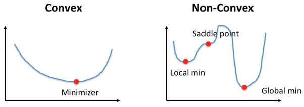
• Convex Cost Functions: These cost functions are bowl-shaped and ideal for optimization using gradient descent. They guarantee global optimality and uniqueness of solutions, enabling more efficient training.

• Non-Convex Cost Functions: Characterized by multiple local minima, maxima, or saddle points, non-convex cost functions can lead optimization algorithms astray, potentially converging to suboptimal solutions.

Convex Cost Functions

For a cost function $J(\theta)$ to be convex, the following inequality holds true for any pair of points $(p, q)$ in the domain:

$$ J( (1-t)p + tq ) \leq (1-t)J(p) + tJ(q) $$

Consequently, if the second derivative of the cost function, i.e., the Hessian matrix, is positive semi-definite for all points within the domain, the function is convex.

Non-Convex Cost Functions

A cost function that violates the aforementioned inequality between points is considered non-convex. This generally occurs because it:

• Suffers from oscillations and irregularities.
• Might contain multiple local minima and maxima.
• Can have saddle points where the first derivative is zero, leading gradient-based optimization to stall.

Practical Implications

The nature of the cost function greatly impacts the suitability of optimization algorithms.

• For convex cost functions, algorithms like gradient descent are more robust and efficient, as they are assured to converge to a global minimum.
• In contrast, non-convex cost functions necessitate more sophisticated approaches, like simulated annealing, genetic algorithms, and heuristic-driven optimization.

Visual Representation

Code Example: Visualizing Convex & Non-Convex Cost Functions

Here is the Python code:

import numpy as np
import matplotlib.pyplot as plt

# Define the range for x
x = np.linspace(-10, 10, 100)

# Define the convex and non-convex cost functions
convex_function = lambda x: (x - 3)**2 + 5
non_convex_function = lambda x: 0.1*x**4 + 0.5*x**3 - 3*x**2 - 2*x + 10

# Plot both cost functions
plt.figure(figsize=(12, 6))
plt.subplot(1, 2, 1)
plt.plot(x, convex_function(x))
plt.title('Convex Cost Function')

plt.subplot(1, 2, 2)
plt.plot(x, non_convex_function(x))
plt.title('Non-Convex Cost Function')

plt.show()

6. Why is convexity important in cost functions?

A convex optimization problem is one in which the objective function and the feasible region are both convex. This characteristic is crucial in the context of machine learning, as it ensures that the optimization techniques used to minimize the cost function consistently converge to the global optimum.

Key Features of Convex Functions

• Local Minima vs. Global Minima: Convex functions have a unique global minimum, making them particularly well-suited for optimization tasks.

• Slope Direction: A straight line connecting any two points on a convex function remains above the function itself. This property underlies the concept of convexity.

• Calculation Simplicity: Derivatives of convex functions are straightforward to compute. A continuous, differentiable, and strictly convex function has a single stationary point, which is a global minimum.

Non-Convexity Challenges

While it's true that not all non-convex functions pose insurmountable optimization problems, the following reasons underscore the preference for using convex functions in many machine learning tasks:

1. Optimization Difficulty: Locating global minima in non-convex functions can be challenging and may require the use of specialized techniques, such as random initialization and potentially multiple runs.

2. Model Interpretability: Constructing and interpreting models based on non-convex cost functions can be intricate and may produce less reliable results.

3. Performance Variability: The performance of non-convex optimizations can be sensitive to the choice of initial parameters and tuning of hyperparameters.

Considering these challenges, the overarching recommendation in machine learning is to work with convex cost functions whenever possible. This strategic choice is key to ensuring the robustness, accuracy, and efficiency of your machine learning models.

7. What is the significance of the global minimum in a cost function?

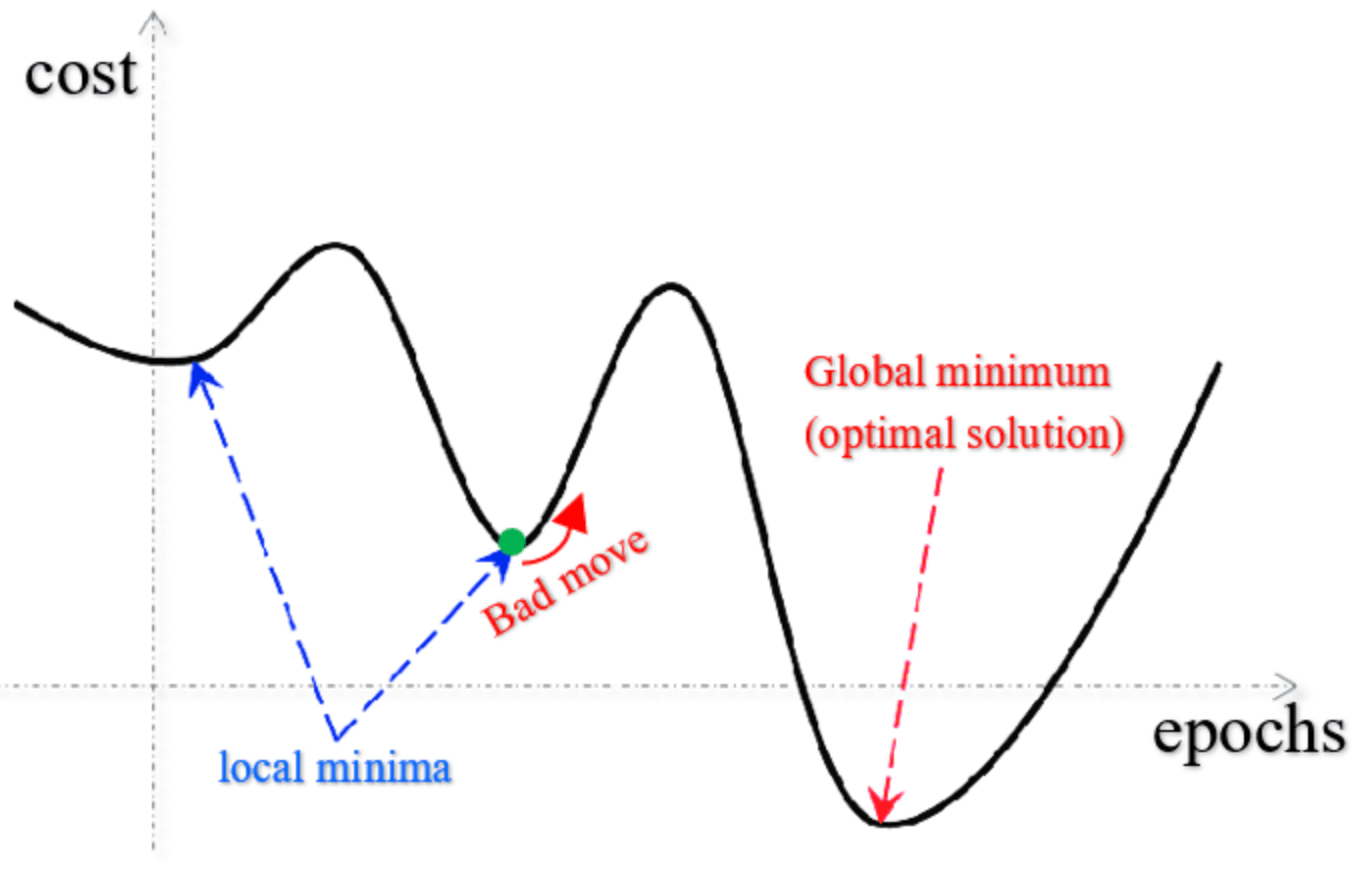
The global minimum in a cost function plays a pivotal role in machine learning, ensuring that your learning algorithm converges to a stable and meaningful solution.

Visualizing Local and Global Minima

Global Minimum: A Focal Point

A cost function plots the cost (or error) against a set of parameters, forming a multi-dimensional space. The parameters influencing the cost function are iteratively manipulated during the training phase.

Several local minima could exist in this space, making it challenging for optimization algorithms. Moreover, the sheer volume of points to consider can be overwhelming.

By aiming to reach the global minimum, machine learning algorithms can effectively refine model parameters, laying the foundation for the desired performance.

Types of Extrema

• Global Minimum: The lowest point in the cost function, defining the most optimal parameter values.
• Local Minimum: Points in the cost function that are lower than all neighboring points, but not necessarily the lowest.

Finding the Global Minimum

Discovering the global minimum involves locating the smallest value across the cost function, irrespective of the starting point or any local minima.

While exploring the multidimensional space defined by the cost function, optimization algorithms seek to identify the global minimum:

1. Direct Method: Exhaustive search over a range of parameter values.
2. Local Refinement: Beginning from an initial guess, iterative updates are made to explore and refine parameter values. This is particularly useful for high-dimensional spaces.
3. Probabilistic Approach: Uses random sampling to estimate the minimum.

However, for high-dimensional cost functions, these methods can be computationally demanding.

The Hinge Loss Example

Take, for instance, the hinge loss function, common in support vector machines:

$$ L(y, f(\mathbf{x})) = \max(0, 1 - y \cdot f(\mathbf{x})) $$

Here, $y$ represents the true label, $\mathbf{x}$ is the input data, $f(\mathbf{x})$ reflects the model's prediction, and $L$ computes the prediction error. The aim is to minimize the sum of these hinge loss values across all data points.

8. How does the choice of cost function affect the generalization of a model?

The cost function is pivotal to both the training and generalization of a model. Its role is especially evident during gradient descent, which aims to find the model's parameters that minimize this function.

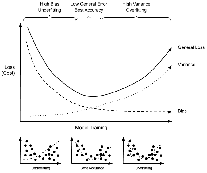
While a simpler cost function, like mean squared error (MSE), can often make the optimization process faster, it might become prone to overfitting. On the other hand, more sophisticated cost functions such as regularized methods can more effectively manage model complexity, thus reducing overfitting and enhancing generalization.

Types of Cost Functions

Unregularized Cost Functions

1. Mean Squared Error (MSE): Measures the average of the squares of the errors between predicted and true values. It's prone to overfitting due to its strong emphasis on correctly predicting outliers.

$$ \text{MSE} = \frac{1}{N} \sum_{i=1}^{N} (y_i - \hat{y}_i)^2 $$

2. Mean Absolute Error (MAE): Averages the absolute differences between predicted and true values. It's more robust against outliers but can slow down training due to its non-differentiability at zero.

$$ \text{MAE} = \frac{1}{m} \sum_{i=1}^{m} |y_i - \hat{y}_i| $$

Regularized Cost Functions

1. Ridge Regression (L2 Norm): Introduces the sum of squares of the model's coefficients as a penalty term, weighted by a hyperparameter $\lambda$. This discourages the model from oversaturating its parameters.

$$ J(\theta) = \frac{1}{2N} \sum_{i=1}^{N} (h_{\theta}(x^{(i)}) - y^{(i)})^2 + \lambda \sum_{j=1}^{n} \theta_j^2 $$

2. Lasso Regression (L1 Norm): Similar to Ridge but uses the sum of the absolute values of the coefficients, acting as a feature selector.

$$ J(\theta) = \frac{1}{2N} \sum_{i=1}^{N} (h_{\theta}(x^{(i)}) - y^{(i)})^2 + \lambda \sum_{j=1}^{n} \left| \theta_j \right| $$

3. Elastic Net: A hybrid of Ridge and Lasso that combines both L1 and L2 norms. It uses both the absolute and squares of the coefficients to penalize the model. This avoids some of the limitations of both methods when used individually.

$$ J(\theta) = \frac{1}{2N} \sum_{i=1}^{N} (h_{\theta}(x^{(i)}) - y^{(i)})^2 + \lambda \left( (1 - r) \sum_{j=1}^{n} \theta_j^2 + r \sum_{j=1}^{n} \left| \theta_j \right| \right) $$

4. Cross-Entropy: Standard for binary classification tasks, it penalizes the model more heavily when confident incorrect predictions are made.

$$ H(p,q) = -\frac{1}{N} \sum_{i=1}^{N} \left( y_i \log(\hat{y}_i) + (1 - y_i) \log(1 - \hat{y}_i) \right) $$

Outliers

The way a cost function treats outliers can deeply influence a model's predictive accuracy. For example, both the Mean Absolute Error (MAE) and the Mean Squared Error (MSE) can be heavily skewed by outliers. While the MAE is less sensitive to such extreme values, the MSE can be significantly influenced by their large squared errors.

Model Complexity and Regularization

The importance of model complexity and its influence on the selection of features and the fit to the data also intersects with the role of a cost function. In response, more evolved cost functions have emerged, like the regularized cost functions. Through the introduction of a regularization term, which varies depending on the model's parameters and aims to penalize the model for its complexity, they can tend to reduce the degree of overfitting and concurrently boost the model's generalizing capacity.

For a clearer understanding, consider the role of the ridge regularization term. This term, as seen below, is a function of the square of all the model's parameters. By scaling these parameters by a factor of the hyperparameter, $\lambda$, discrepancies between the scale of features, and even dimensions numerous folds apart, can be alleviated. This assuages the risk of the model fitting too intensely to a specific feature due to its larger scale or appreciable abundance.

$$ \text{ridge regularization term} = \lambda \sum_{i=1}^{N} \theta_i^2 $$

Balancing Trade-Offs

The choice of cost function is hence a multi-faceted decision that should factor in the peculiarities of the dataset, the specific task at hand, and the model's architecture. Finding a middle ground is frequently paramount as models are commonly judged on their generalizing durabilities. A model that identifies too closely with the provided data but performs sub-optimally when presented with a novel but similar dataset is an issue in need of remedy. This can happen when a model has been overfit, which is a kind of dysfunctional state that results from trying too hard to reveal the subtleties of the training dataset.

9. Describe the Mean Squared Error (MSE) cost function and when to use it.

The Mean Squared Error (MSE) cost function is commonly used in regression tasks, providing a straightforward method for assessing model accuracy.

Math Behind It

MSE calculates the average of the square differences between the predicted and actual output:

$$ MSE = \frac{1}{n} \sum_{i=1}^{n} (y_{\text{actual}} - y_{\text{predicted}})^{2} $$

where:

• $n$ is the number of samples
• $y_{\text{actual}}$ is the actual target value
• $y_{\text{predicted}}$ is the predicted target value

Key Considerations

• Calculation Simplicity: Squaring the differences forces all values to be positive, simplifying calculations.

• Emphasis on Outliers: Squaring can significantly amplify the influence of larger errors, making it sensitive to outliers.

• Units Consistency: The MSE, when used with consistent units, produces an error metric in the same units, thereby aligning well with practical interpretations.

• Derivation: Minimizing the MSE with respect to model parameters leads to the "ordinary least squares" (OLS) method.

• Limitations in Interpretation: While it's easy to interpret, say, that an MSE of 10 means the model's predictions are off by 10 units on average, understanding the practical impact of that could be difficult. Additionally, due to most observations being concentrated around the prediction, the average square error might look deceptively small.

Code Example: Calculate MSE

Here is the Python code:

from sklearn.metrics import mean_squared_error

# Assuming y_true and y_pred are available
mse = mean_squared_error(y_true, y_pred)
print("Mean Squared Error:", mse)

10. Explain the Cross-Entropy cost function and its applications.

Cross-entropy is a cost function used in classification tasks, especially when dealing with probabilities. It's particularly well-suited for binary classifications.

Cross-Entropy Cost Function

In the two-class scenario, the output of the $\sigma$ function, or the logistic function, can be either the predicted probability that the sample belongs to class 1, or class 0.

Using the logistic function, $\sigma(t) = \frac{1}{1+e^{-t}}$, we convert the model's output to the range $(0, 1)$, representing probabilities.

The cost function is derived straightforwardly from the likelihood that the observed result $y$ is drawn from a distribution described by $\sigma(t)$:

$$ \begin{equation} \begin{split} \text{Cost}(y, \hat{p}) = \begin{cases} -\log(\hat{p}) & \text{if } y = 1 \ -\log(1 - \hat{p}) & \text{if } y = 0 \end{cases} \end{split} \end{equation} $$

An equivalent, more concise, formulation of the cross-entropy cost function:

$$ \text{Cost}(y, \hat{p}) = -y \log(\hat{p}) - (1 - y)\log(1 - \hat{p}) $$

Here, $\hat{p}$ is the predicted probability and $y$ takes the value 0 or 1.

Code Example: Cross-Entropy in Python

Here is the Python code:

import numpy as np

def cross_entropy(y, p_hat):
    return -y * np.log(p_hat) - (1 - y) * np.log(1 - p_hat)

# Example usage
y_true = 1
p_predicted = 0.9
cost = cross_entropy(y_true, p_predicted)
print(cost)

11. What is the Hinge loss, and in which scenarios is it applied?

Hinge Loss serves as a margin-based cost function for binary classification tasks. It is a key component in the Support Vector Machine (SVM) learning algorithm.

Visual Representation

Mathematical Representation

The Hinge Loss function $L(y, \hat{y})$ is defined as:

$$ L(y, \hat{y}) = \max(0, 1 - y \cdot \hat{y}) $$

Where:

• $y$ is the true class label (either -1 or 1)
• $\hat{y}$ is the predicted class label
• $y \cdot \hat{y}$ is the dot product of $y$ and $\hat{y}$

Core Concept: Margin

The Hinge Loss is built around the concept of a "margin," which is effectively the confidence in the model's classification. A larger margin means higher confidence.

• If $y \cdot \hat{y} \geq 1$, the predicted class is correct, and the loss is 0.
• If $y \cdot \hat{y} < 1$, the predicted class is incorrect, and the loss increases with the decrease in the margin.

Application: Support Vector Machines (SVM)

In the context of SVM:

• The loss term encourages the model to correctly classify samples, especially those close to the decision boundary.
• It introduces a hard margin, meaning that any misclassification incurs the same penalty, regardless of distance from the boundary.

12. How is the Log Loss function used in logistic regression?

Logistic regression uses the Log Loss (cross-entropy) function as its cost function, optimizing model parameters through gradient descent.

This form of cost function best suits the probabilistic nature of binary classification tasks.

Advantages of Log Loss in Binary Classification

• Sensitivity: Log Loss is more sensitive to mistakes in extreme probabilities, emphasizing their differentiation. For instance, it penalizes a confident wrong prediction more.
• Probabilistic Interpretation: As Log Loss measures the difference between probability distributions, it's a natural fit for probability-based models like logistic regression.
• Derivatives: The function's smoothness and well-defined derivatives simplify optimization using gradient-based methods.

Mathematical Formulation

The Log Loss function is defined as:

$$ \text{Log Loss} = -\frac{1}{N}\sum_{i=1}^{N}[y_i\log(p_i) + (1-y_i)\log(1-p_i)] $$

Here:

• $N$ is the number of samples.
• $p_i$ is the predicted probability of class 1 for the $i$-th sample.
• $y_i$ is the actual class label of the $i$-th sample (0 or 1).

Code Example: Log Loss Calculation

Here is the Python code:

import numpy as np

def log_loss(y_true, y_pred):
    epsilon = 1e-15  # Small value to avoid potential divide-by-zero errors
    y_pred = np.clip(y_pred, epsilon, 1 - epsilon)  # Clip values to be within 0-1
    N = len(y_true)
    loss = -1/N * np.sum(y_true * np.log(y_pred) + (1-y_true) * np.log(1-y_pred))
    return loss

# Example usage
y_true = np.array([1, 0, 1, 1])
y_pred = np.array([0.9, 0.2, 0.85, 0.99])
print("Log Loss:", log_loss(y_true, y_pred))

13. Discuss the role of the Huber loss and where it is preferable over MSE.

The Huber Loss represents a compromise between the Mean Absolute Error (MAE) and the Mean Squared Error (MSE) and is often chosen for its resilience against outliers.

Outlier Sensitivity in Loss Functions

Some loss functions are more sensitive to outliers than others:

• MAE: All data points have equal influence.
• MSE: Squares the errors which gives more emphasis on the larger errors, making it sensitive to outliers.
• Huber Loss: Adaptable near the origin to be less sensitive to outliers, and like MAE as the error grows large.

The Huber Loss provides a balanced approach by having both a linear and a quadratic term, switching between the two based on a predefined threshold. This provides the best of both worlds:

1. Robustness: The linear regime is less influenced by outliers, and
2. Efficiency: The quadratic regime deals effectively with inliers.

Mathematical Representation

The Huber Loss combines linear and quadratic functions:

$$ L_{\text{Huber}} = \begin{cases} \frac12 x^2 & \text{for } |x| \leq \delta \\ \delta (|x| - \frac12 \delta) & \text{for } |x| > \delta \end{cases} $$

Here, $\delta$ represents the threshold where the function switches from a quadratic to a linear operation.

Code Example: Huber Loss

Here is the Python code:

import numpy as np

def huber_loss(y_true, y_pred, delta=1.0):
    """Calculates the Huber Loss."""
    residual = y_true - y_pred
    abs_residual = np.abs(residual)
    
    # Calculate loss based on the defined thresholds
    quadratic_part = np.minimum(abs_residual, delta)
    quadratic_part = 0.5 * quadratic_part ** 2
    linear_part = abs_residual - delta
    linear_part = delta * linear_part - 0.5 * delta ** 2
    
    # Choose the loss component based on the thresholds
    loss = np.where(abs_residual <= delta, quadratic_part, linear_part)
    
    return np.mean(loss)

# Example usage
y_true = np.array([1, 2, 3, 4, 5])
y_pred = np.array([2, 2, 3, 5, 8])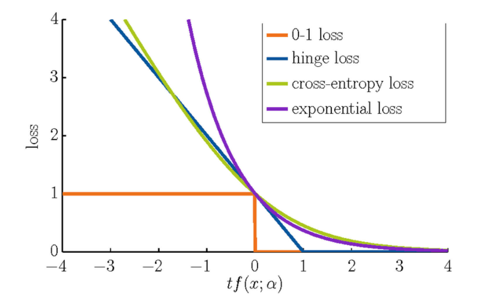
print("Huber Loss:", huber_loss(y_true, y_pred, delta=1.0))

14. What is the 0-1 loss function, and why is it often impractical?

The 0-1 loss function, which is also known as the classification error, is a simple and intuitive way to measure the misclassification error in Machine Learning tasks.

Function

Here is formal way to define it (note that this is not a convex function):

$$ I(y \neq \hat{y}) = \begin{cases} 0 & \text{if } y = \hat{y} \\ 1 & \text{if } y \neq \hat{y} \end{cases} $$

Limitations

While mathematically straightforward, the 0-1 loss function has practical limitations when used with optimization algorithms like gradient descent due to the following reasons:

1. Non-convexity: It is a non-convex function, characterized by multiple local minima, which can hinder the convergence of optimization algorithms.
2. Discontinuity: The sudden jump from 0 to 1 at the decision boundary makes the function non-differentiable, causing difficulties for gradient-based optimization methods which rely on derivatives.
3. Zero Gradients: The function has zero gradients almost everywhere, except at the decision boundary, making it challenging for algorithms to identify a clear direction for improvement.

Practical Alternatives

To address the limitations of the 0-1 loss function, a common practice is to use surrogate losses, such as the logistic loss (binary cross-entropy), hinge loss, or squared loss for logistic regression or other classification tasks, which are better suited for optimization techniques like gradient descent.

15. Explain the concept of Regularization in cost functions.

Regularization in machine learning aims to prevent overfitting by reducing the complexity of a model.

Purpose of Regularization

• Oversimplification: Models without tuning or regularization might be too simplistic, resulting in underperforming on unseen data.
• Overfitting: This occurs when a model learns to fit the training data so well that it doesn't generalize to new data. Overfitting can stem from the model trying to capture noise in the data, or when it's too complex relative to the amount of training data available.

Regularization imposes a penalty for model complexity to steer the model towards a sweet spot, balancing the goodness of fit with the model's complexity.

Types of Regularization

• $L1$ regularization: This method adds the sum of the absolute weights to the cost function. It is useful for feature selection.
• $L2$ regularization: This method adds the sum of the squared weights to the cost function. It is useful for preventing overly large weights that might lead to overfitting.

Cost Function Modifications

In the context of linear regression, the cost function represents the mean squared error. Regularization entails modifying this cost function with an added term reflecting the chosen regularization method.

The general form of the modified cost function, denoted as J tilde, is:

J tilde = J + alpha * reg_term

Where:

• J represents the standard mean squared error or cost function.
• alpha is the regularization parameter, a non-negative value that controls the influence of the regularization term. Typically, it's selected via techniques like cross-validation.
• reg_term is a function of the model's weights that we compute based on the chosen regularization method.

Code Example: Regularized Linear Regression

Here is the Python code:

import numpy as np

# Create sample data
np.random.seed(0)
X = np.random.rand(100, 1)
y = 2 + 3 * X + np.random.randn(100, 1)*0.5

# Add polynomial features (up to degree 3)
from sklearn.preprocessing import PolynomialFeatures
poly_features = PolynomialFeatures(degree=3, include_bias=False)
X_poly = poly_features.fit_transform(X)

# Train the model
from sklearn.linear_model import Ridge
ridge_reg = Ridge(alpha=1, solver="cholesky")
ridge_reg.fit(X_poly, y)

# Make predictions using the model
y_predictions = ridge_reg.predict(X_poly)

# Visualize the model predictions
import matplotlib.pyplot as plt
plt.scatter(X, y, color='blue')
plt.plot(X, y_predictions, color='red')
plt.show()

In this example, Ridge regression is used with an $L2$ regularization term. The alpha parameter controls the degree of regularization.

Explore all 43 answers here 👉 Devinterview.io - Cost Function