You can install scMEGA via below commands:
# Install devtools
if (!requireNamespace("devtools", quietly = TRUE))
install.packages("devtools")
# First install Seurate v5
devtools::install_github("satijalab/seurat", "seurat5", quiet = TRUE)
# Install Signac
devtools::install_github("stuart-lab/signac", "seurat5")
# Install scMEGA
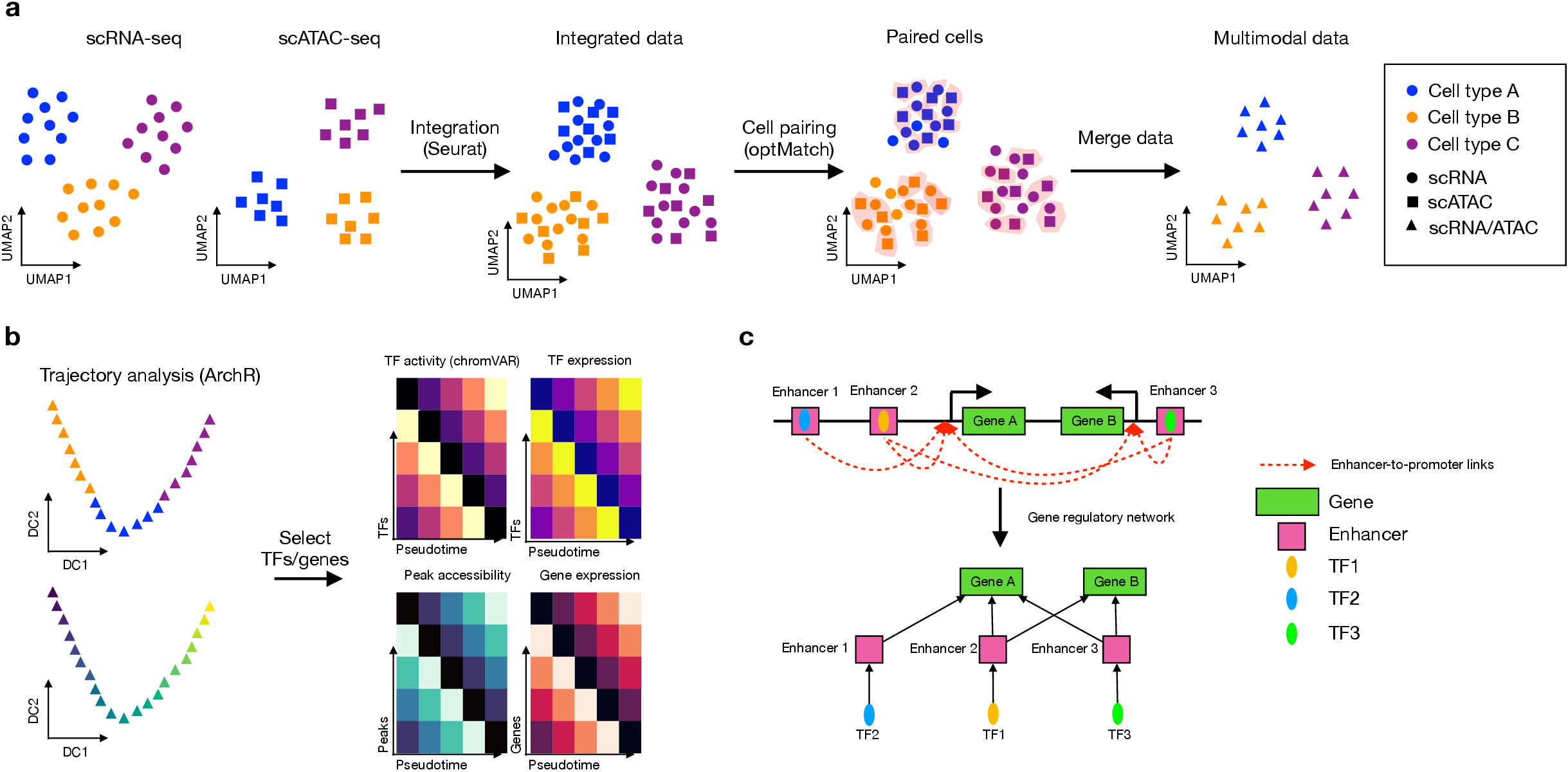
devtools::install_github("CostaLab/scMEGA")We provided the following tutorials to show how to use scMEGA to build GRN by using single-cell multiomics/multimodal data:
Please consider citing our paper if you used scMEGA:
@article{li2023scmega,
  title={scMEGA: single-cell multi-omic enhancer-based gene regulatory network inference},
  author={Li, Zhijian and Nagai, James S and Kuppe, Christoph and Kramann, Rafael and Costa, Ivan G},
  journal={Bioinformatics Advances},
  volume={3},
  number={1},
  pages={vbad003},
  year={2023},
  publisher={Oxford University Press}
}


