camachodejay / fret-calculations

This repository contains the code necessary to simulate the fluorescence emission of an anisotropic ensemble of GFP molecules when excited by polarized light.

FRET-calculations

This repository contains the code necessary to simulate the fluorescence emission of an anisotropic ensemble of GFP molecules when excited by polarized light. This simulation is part of the manuscript entitled: 2D polarization imaging as a low-cost fluorescence method to detect α-synuclein aggregation ex vivo in models of Parkinson’s disease. By Rafael Camacho, Daniela Täuber, Christian Hansen, Juanzi Shi, Luc Bousset, Ronald Melki, Jia-Yi Li, and Ivan G. Scheblykin.

Figure 01: Definition of energy funneling efficiency ε (top panel) and calculations of the fluorescence anisotropy r and ε as functions of the distance between GFP molecules in a cubic lattice (bottom panel). The homo-FRET Förster radius for GFP is 4.7 nm according to its spectral properties. On the right column pictograms of: a monomer, b dimer, c densely, and d loosely packed aggregates of α-syn-GFP. The monomer/dimer ratio indicates how many sites of the lattice are occupied by a monomer/dimer. Black arrows show the transition from the pure monomer to the pure dimer case. Error bars represent the standard deviation of the simulations when repeated 10 times.

In the simulations we consider the presence of homo-FRET between GFP molecules. The simulation pipeline can be seen as:

1. Generation of dipole model
   1. Dipole positions
   2. Dipole orientations
   3. calculation of the FRET rate between all dipoles
2. Generation of the polarization portrait
   1. Calculation of the steady state transfer matrix
   2. Calculation of the fluorescence intensity response
3. Calculation of the POLIM output from the polarization portrait

• Version release-01, as used in the article.
• Website of the author

How do I get set up?

• Summary of set up: This is a Matlab repository. Thus, you will need to have a local Matlab installation. To run the code just run the main function.
• Configuration: NA.
• Dependencies: NA.

Contribution guidelines

• If you wish to contribute to this project please email the author.

Who do I talk to?

• If you ever encounter a problem feel free to contact the author Website of the author

• For information related to the article feel free to reach the author and/or Prof. Ivan Scheblykin

Detailed information about the code

The code is written using the object-oriented-programming capabilities of Matlab. There are 2 main objects:

1. +Dipole.dipole_model: This one contains all the information about dipole positions, orientations, and FRET rate between dipoles.
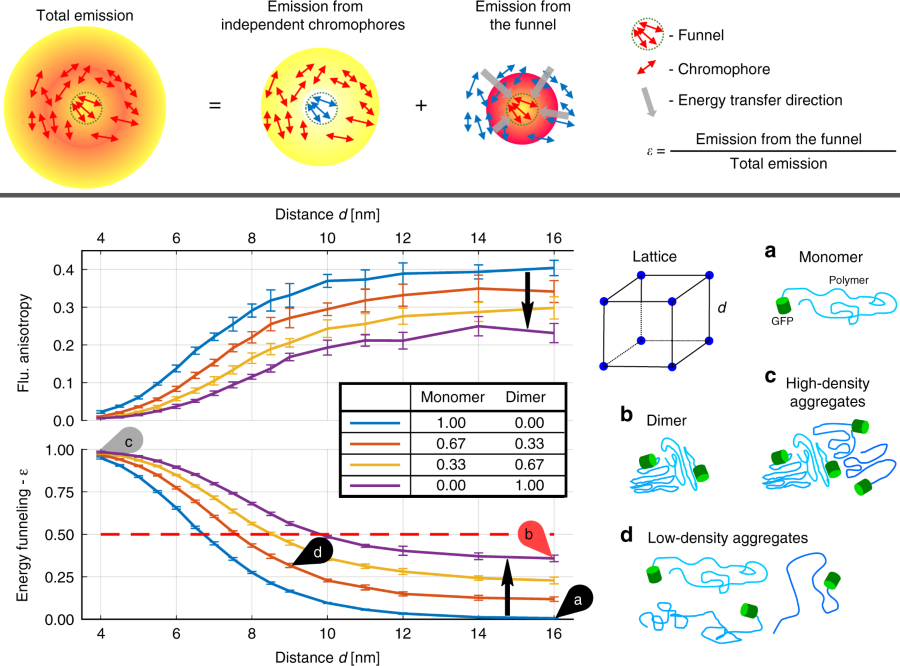
2. +Portrait.pol_portrait: This one calculates the steady state emission of the system after the FRET process has taken place. With that information it then calculates the polarization portrait for the model system. Once the portrait is known then we can calculate the POLIM parameters, such as, modulation depths and phases in excitation and emission, fluorescence anisotropy, and energy funnelling parameter - epsilon.

How does the simulation work

A dipole model object contains the positions of all dipoles in the model system. The positions start with a central dipole in the origin (x: 0, y:0, z:0) surrounded by a large number of buffer dipoles in a cubic lattice, where all dipoles are randomly oriented. The central dipole is the dipole of interest for which the excitation/emission properties will be calculated. The buffer dipoles can be seen as a bath affecting the response of the central dipole depending on their positions/orientation.

This means that each time we simulate a dipole model the polarization portrait we obtain has fully polarized excitation (single absorbing dipole) and emission polarization that depends on the interaction between the central dipole and its buffer. If the buffer dipoles are far away (tens of nm) then they do not affect the central dipole and emission will also be fully polarized. On the other hand, if the buffer dipoles are very close (<4 nm), then the energy absorbed by the central dipole will be transferred and completely redistributed into the bath making the emission anisotropic.

Now, in order to simulate the response coming from a set of randomly oriented dipoles (e.g. GFP in solution) many (thousands) of dipole model iterations have to be done. This is because by adding together the response of many single_dipole-bath systems we obtain the response coming from a large set dipoles randomly orientated in the 3D.

What about the presence of dimmers? to consider the effects of dimers in the polarization properties of the system we do the following: We randomly take a fraction of the sites in the cubic lattice and replace their monomer by a model dimer. This model dimer consists of two dipoles with the following properties:

1. The two dipoles are separated by a fixed distance (dimer distance).
2. The center of gravity of the model dimer is set to the original cubic lattice position.
3. The relative orientation of the dipoles inside the dimer is random.
4. The position of the dipoles relative to their center of mass is also random.

How do we calculate the transfer rate between dipole? We follow the classical FRET equations based in the distance/orientation and the spectral overlap between the donor and acceptor(s). For more details see information below.

Dipole model

• Description: Object that contains the positions, orientations and transfer matrix of all dipoles in the model system. The list of positions contains a central dipole in the origin surrounded by a large number of buffer dipoles in a cubic lattice. All dipoles are randomly oriented. There is the option of replacing the monomer sites by a dimer.

• Properties:

  1. distance_model: string that tells the object what kind of lattice we are going to build, 1D a line, 2D a plane, 3D a cube.
  2. buffer: structure that contains information about buffer dipoles. max_n_dipoles: maximum number of dipoles in the system; max_size maximum desired size of the buffer in nm; min_size: minimum desired size of the buffer in nm.
  3. buffer_used: size of the actual buffer used in nm.
  4. positions: list of positions of all dipoles in the system in cartesian coordinates.
  5. orientations: list of unitary vectors that point in the direction of the dipoles in the system.
  6. transfer_matrix: matrix that contains the transfer rate between all dipoles in the system. Elements in the diagonal express how much light remains in the dipole and thus is emitted as fluorescence. Note that this matrix considers a single step energy transfer process, it is not the steady state transfer matrix.
  7. central_dipole: index of the central dipole in the positions/orientations matrices.

• Methods:

  1. object constructor D = Dipoles.dipole_model(dist_model, buffer);: dist_model must be a string '1D', '2D' or '3D'. buffer must be a structure with fields 'max_n_dipoles','max_size' and 'min_size'. size parameters are in units of nm. The object constructor returns an initialized dipole_model system.
  2. get_positions D = D.get_positions(inter_dist, dimer_prob): inter_dist double containing the inter chromophoric distance in nm; dimer_prob double with value between 0-1 that contains the probability for a site in the cubic lattice to contain a dimer instead of a monomer. It returns a dipole_model object with positions, buffer_used and central_dipole properties filled in.
  3. get_orientations D = D.get_orientations(): If the dipole_model 'D'contains a list of positions then it returns a dipole_model object with orientations filled in.
  4. get_et_matrix D = D.get_et_matrix(FRETprops): FRETprops is a structure with fields 'J', 'extinction_coef', 'lifetime_donor', 'quantum_yield' and 'refractive_index'. If the dipole_model 'D' contains a list of positions and orientations then it returns a dipole_model object with et_matrix filled in.

• Detailed Explanation here I'm planning to explain each step of the code if possible.

Polarization portrait

• Description:Object that contains the polarization portrait and all the information needed to create it. This includes translation of the one step transfer matrix into steady state emission after all transfer steps have taken place.

• Properties:

  1. ex_angles_rad: vector of doubles containing the discrete excitation angles in radians used to create the polarization portrait.
  2. em_angles_rad: vector of doubles containing the discrete emission angles in radians used to create the polarization portrait.
  3. et_steps: number of times one step transfer matrix had to be used in order for all the initial excitation energy to decay via emission. In other words how many energy transfer steps the dipole model had.
  4. res_ener: Our estimation for the steady state emission after FRET is a numerical calculation. This means that I keep doing ET steps until 'most' of the energy is gone via emission. res_ener keeps track of how much residual energy was left in the system when I stoped the calculation due to numerical reasons.
  5. I_ex_em: polarization portrait, fluorescence intensity as function of the excitation and emission polarization angles.
  6. em_after_et: Numerically estimated steady state emission after FRET for the central dipole.

• Methods:

  1. object constructor P = Portrait.pol_portrait(dipole_model, portrait_prop): dipole_model must be a dipole model object with defined positions, orientations, and et_matrix; portrait_prop must be a structure with fields 'em_angles' and 'ex_angles', which should be each a 1xn array containing angles in degrees. The constructor then calculates the polarization portrait for the given dipole model (only the response of the central dipole!).
  2. display_portrait P.display_portrait(): generates a new Matlab figure and plots (contour plot) the polarization portrait.

• Detailed Explanation here I'm planning to explain each step of the code if possible.

POLIM calculation

For a detailed explanation please follow the links below:

• Quantitative characterization of light-harvesting efficiency in single molecules and nanoparticles by 2D polarization microscopy: Experimental and theoretical challenges

• Fluorescence polarization measures energy funneling in single light-harvesting antennas—LH2 vs conjugated polymers

• Polarization portraits of light-harvesting antennas: from single molecule spectroscopy to imaging