abelfunctions / abelfunctions

A library for computing with Abelian functions, Riemann surfaces, and algebraic curves.

Abelfunctions

A Sage library for computing with Abelian functions, Riemann surfaces, and algebraic curves. Abelfunctions is the Ph.D. thesis work of Chris Swierczewski. (GitHub: cswiercz). Abelfunctions requires Sage 9.2 or later.

sage: from abelfunctions import *
sage: R.<x,y> = QQ[]
sage: X = RiemannSurface(y**3 + 2*x**3*y - x**7)
sage: X.riemann_matrix()
array([[-1.30901699+0.95105652j, -0.80901699+0.58778525j],
       [-0.80901699+0.58778525j, -1.00000000+1.1755705j ]])
sage: P = X(0)[0]; P
(t, 1/2*t^4 + O(t^7))
sage: AbelMap(P)
array([-0.29124012+0.64492948j, -0.96444625+1.1755705j ])
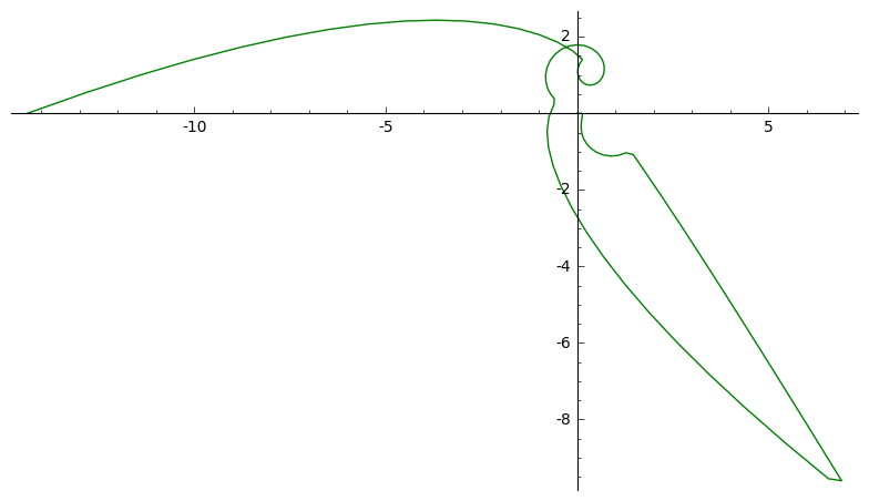
sage: gamma = X.path(P)
sage: gamma.plot_x(); gamma.plot_y(color='green');

Documentation and Help

For installation instructions, tutorials on how to use this software, and a complete reference to the code, please see the Documentation. You can also post questions in the Discussions Page.

Please report any bugs you find or suggest enhancements on the Issues Page.

Extensions to Abelfunctions

• CyclePainter - A tool for building custom paths on Riemann surfaces

Citing this Software

C. Swierczewski et. al., Abelfunctions: A library for computing with Abelian functions, Riemann surfaces, and algebraic curves, http://github.com/abelfunctions/abelfunctions, 2017.

BibTeX:

@misc{abelfunctions,
  author = {C. Swierczewski and others},
  title = {Abelfunctions: A library for computing with Abelian functions, Riemann surfaces, and algebraic curves},
  note= {\tt http://github.com/abelfunctions/abelfunctions},
  year = 2017,
}

abelfunctions's Issues

X.place() Doesn't Return Enough Places

Example:

Input:

import abelfunctions
from sympy.abc import x,y
f = -x**7 + 2*x**3*y + y**3
X = ab.RiemannSurface(f,x,y)
b = X.discriminant_points()
b0 = b[2]

places = X(b0)
for P in places:
    print P
    print

Output:

x(t) = 2*RootOf(27*x**5 + 1, 0) + (1)t**1
y(t) =  + (-8*3**(3/5)/9) + ((448*RootOf(27*x**5 + 1, 0)**6 + 64*3**(3/5)*RootOf(27*x**5 + 1, 0)**2/3)/(16*RootOf(27*x**5 + 1, 0)**3 + 64*3**(1/5)/9))t**1 + O(t**2)

This is incorrect since the sum of the ramification indices of all places lying above any x=a must equal the y-degree of the curve.

Possible error locations include:

• abelfunctions.RiemannSurface.__call__()
• abelfucntions.divisiors.Place.__init__()
• abelfunctions.puiseux.puiseux()

If it's the latter it's probably because of the use of the SymPy's RootOfconstruct.

Skip puiseux at regular points

The only x-points where we need to use puiseux.puiseux() to calculate a local series expansion are the discriminant points and infinity. At all other points we should be able to skip straight to using puiseux.newton_iteration() like so:

In [1]:

f = x**2*y**3 - x**4 + 1

# uses puiseux
places = abelfunctions.puiseux.puiseux(f,x,y,2,order=4)
for P in places:
    print P
    print

Out[1]:

x(t) = 2 + (1)t**1
y(t) =  + (2537*30**(1/3)/109350)t**3 + (-571*30**(1/3)/16200)t**2 + (17*30**(1/3)/90)t**1 + (30**(1/3)/2) + O(t**4)

x(t) = 2 + (1)t**1
y(t) =  + (-10148*10**(1/3)/(72900*3**(2/3) - 218700*3**(1/6)*I))t**3 + (15417*10**(1/3)/(72900*3**(2/3) - 218700*3**(1/6)*I))t**2 + (-82620*10**(1/3)/(72900*3**(2/3) - 218700*3**(1/6)*I))t**1 + (-218700*10**(1/3)/(72900*3**(2/3) - 218700*3**(1/6)*I)) + O(t**4)

x(t) = 2 + (1)t**1
y(t) =  + (-10148*10**(1/3)/(72900*3**(2/3) + 218700*3**(1/6)*I))t**3 + (15417*10**(1/3)/(72900*3**(2/3) + 218700*3**(1/6)*I))t**2 + (-82620*10**(1/3)/(72900*3**(2/3) + 218700*3**(1/6)*I))t**1 + (-218700*10**(1/3)/(72900*3**(2/3) + 218700*3**(1/6)*I)) + O(t**4)

In [2]:

places[2].eval_y(t).simplify().collect(t,evaluate=False)

Out[2]:

{t**2: 571*30**(1/3)/32400 - 571*10**(1/3)*3**(5/6)*I/32400,
 t**3: -2537*30**(1/3)/218700 + 2537*10**(1/3)*3**(5/6)*I/218700,
 1: -30**(1/3)/4 + 10**(1/3)*3**(5/6)*I/4,
 t: -17*30**(1/3)/180 + 17*10**(1/3)*3**(5/6)*I/180}

In [3]:

alphas,betas = zip(*X(2))
G = f.subs({x:(2+t), y:(betas[0]+y)})
abelfunctions.puiseux.newton_iteration(G,t,y,4).simplify().collect(t,evaluate=False)

Out[3]:

{t**2: 571*30**(1/3)/32400 - 571*10**(1/3)*3**(5/6)*I/32400,
 t**3: -2537*30**(1/3)/218700 + 2537*10**(1/3)*3**(5/6)*I/218700,
 t: -17*30**(1/3)/180 + 17*10**(1/3)*3**(5/6)*I/180}

The above calculation is just confirmation that an appropriate constant shift (to center at (0,0)) and use of newton_iteration() is equivalent to and faster than using puiseux(). On one hand this could be incorporated into puiseux() itself but it requires knowing the discriminant points of f which is done on Riemann surface instantiation.

Investigate Voronoi Decomposition Approach to Computing X-Skeleton

MAGMA's approach to computing period matrices involves computing the Voronoi decomposition of the critical (discriminant) x-points of the curve and integrating the differentials along its edges. That is, path selection along the x-plane is done along the edges of this graph. Currently, a heuristic approach is taken in avoiding the discriminant points.

This would be a nice way to test if XPathFactory is abstract (read: well-written) enough such that the Voronoi approach is easily swappable with the current factory subclass.

Pros

• not heuristic
• (more)

Cons

• Puiseux series convergence is slow. May make taking paths to discriminant places difficult.
• (more)

Implement is_hyperelliptic().

RiemannSurface.is_hyperelliptic() should be easy. Do it.

Possible Bug in Riemann Theta integer_points()?

A bug in the Sage version of the code resulted in imaginary radii. A minor change helped resolve the issue but I'm not sure if it's completely mathematically correct. (Read: I haven't performed the derivations and calculations line-by-line.) Take a look at the calculation of newR in the find_integer_points() subroutine of RiemannTheta.integer_points().

Analytic Continuation along Discriminant Paths Still Buggy

There is a strange (finite) jump at the end of the path.

f = -x**7 + 2*x**3*y + y**3
X = ab.RiemannSurface(f2,x,y)
print X

b = X.discriminant_points()
for bi in b:
    print bi
b0 = b[3]

places = X(b0)
for P in places:
    print P
    print

gamma = X.path(P)

omega = X.holomorphic_differentials()
for om in omega:
    print om

fig = om.plot(gamma,128,True)
ax = fig.gca()
ax.axis([0,1,-.3,.1])
fig.show()

Add option to compute puiseux() up to a degree bound.

puiseux() compute Puiseux series up to a certain number of terms. Add the option to compute the series up to a degree bound instead.

Streamline Integral Basis Riemann Surface Usage

This issue applies to the refactor-algebra branch.

The functions integral_basis(), _integral_basis_monic(), and compute_bd() in the integralbasis module switch back and forth between using a RiemannSurface-like object and using the curve data f = f(x,y) attributes within the object. This constitutes messy code.

The main reason why this "hack" is used is because (currently) puiseux.puiseux() uses a RiemannSurface object as input. The function's only use of Riemann surface is to extract the curve attribute data.

Consider rewriting puiseux.puiseux() to accept only a curve. This probably makes sense mathematically because the definition of the variables used in the Puiseux series representation are obtained from an affine projection of the surface, itself.

Implement Abel Map

Implement the Abel Map. There are two primary situations that need to be considered.

• Abel map to "regular place".
• Abel map to "singular point". (Defined as a place on the Riemann surface where a Puiseux series representation is necessary to distinguish the place from others with the same x-coordinate when parameterized by a complex curve f = f(x,y).)

monodromy() cannot handle single finite discriminant point case

mondoromy:monodromy_graph() throws multiple errors when encountering the case of a single finite discriminant point, such as in the example f(x,y) = x**2 - x*y**2 + y**4.

In Maple, a monodromy group is returned which includes the branch point at infinity. However, a call to homology returns the error:

Warning, negative genus so the curve is reducible
Error, (in algcurves/Canonicalbasis) monodromy not transitive, so curve is reducible

After some experimentation, it seems that a small refactor is needed to resolve this issue cleanly.

Compute Integral Basis

Add functionality to compute integral basis.

Write Separate Subroutine for Constructing non-Parametric Puiseux Series from Parametric Form

In puiseux.py:build_series() the non-parametric forms of the Puiseux series are computed depending on the value of the argument parametric. It would be best to separate this construction / decision out into a separate subroutine for efficiency purposes.

The primary reason for this is so that it's very fast to compute the non-parametric form after computing the parametric form, once function cacheing is implemented. Such situations arise in several applications, such as computing the delta invariant in singularities.py:delta_invariant().

For example,

P = puiseux(f,x,y,alpha,nterms=3,parametric=t)   # normal run-time
Px = puiseux(f,x,y,alpha,nterms=5)               # fast, due to cacheing

Refactor Algebraic Components

The motivation behind refactorization of the algebraic side is two-fold.

1. Puiseux series are not being properly evaluated / manipulated by Sympy.
2. Performance improvements.

Fixing (1) should contribute significantly to (2). This is also a necessary component to implementation of the Abel Map.

Improve xpath_factory.py Documentation

Fix up the documentation for xpath_factory.py. In particular,

• @cswiercz Clean up and expand module-level docstring.
• @mkaralus Clean up class-level docstrings.
  • One-sentence short description.
  • Omit method descriptions from class-level method list. (They should be auto-generated from the one-sentence short description of the method.)
• @mkaralus Add missing Returns sections to appropriate class methods.
  • In general, make sure the numpydoc requirements are satisfied throughout the code. I've been slightly inconsistent with my syntax, etc.
• @mkaralus Add module to "Reference" section in documentation.
• @cswiercz Address todos in code.
• @cswiercz At least add some module-level documentation. (Especially since this code is mostly mature.)

_Note to New Developers_

Be sure to create a new branch with the name of this issue under the dev branch so it's easy to share changes back and forth.

Improve Test Suite

Improve upon the abelfunctions test suite using the unittest module. Some basics are already in place but some investigation in how to make the testing more informative is needed.

Improve Performance of Differentials

Performance report from Commit 0a4952d

Sun Nov 16 21:18:17 2014    differentials.profile

         13056880 function calls (12255645 primitive calls) in 32.782 seconds

   Ordered by: internal time
   List reduced from 1816 to 15 due to restriction <15>

   ncalls  tottime  percall  cumtime  percall filename:lineno(function)
296799/202036    2.552    0.000   15.184    0.000 cache.py:78(wrapper)
1599017/1599016    1.353    0.000    1.359    0.000 {isinstance}
112278/7436    1.159    0.000    3.909    0.001 expr.py:2788(_expand_hint)
86296/83164    1.156    0.000    2.104    0.000 basic.py:333(__eq__)
   179980    0.783    0.000    0.993    0.000 densebasic.py:698(dmp_zero_p)
   353501    0.782    0.000    1.128    0.000 numbers.py:400(__hash__)
   286575    0.769    0.000    2.189    0.000 numbers.py:1708(__hash__)
321617/320449    0.750    0.000    1.525    0.000 sympify.py:52(sympify)
   335623    0.657    0.000    1.677    0.000 numbers.py:1395(__hash__)
   364343    0.639    0.000    0.639    0.000 {hasattr}
687412/646151    0.620    0.000    0.771    0.000 basic.py:100(__hash__)
251678/98342    0.458    0.000    0.655    0.000 basic.py:1847(_preorder_traversal)
   175056    0.456    0.000    0.665    0.000 numbers.py:1554(__new__)
7436/6095    0.439    0.000    7.135    0.001 mul.py:95(flatten)
 5766/421    0.380    0.000    2.788    0.007 simplify.py:2451(powsimp)


Sun Nov 16 21:18:17 2014    differentials.profile

         13056880 function calls (12255645 primitive calls) in 32.782 seconds

   Ordered by: cumulative time
   List reduced from 1816 to 15 due to restriction <15>

   ncalls  tottime  percall  cumtime  percall filename:lineno(function)
        1    0.000    0.000   32.951   32.951 {abelfunctions.differentials.differentials}
        1    0.001    0.001   32.905   32.905 differentials.pyx:108(differentials)
        3    0.000    0.000   18.622    6.207 integralbasis.py:183(integral_basis)
        3    0.001    0.000   17.274    5.758 integralbasis.py:226(_integral_basis_monic)
296799/202036    2.552    0.000   15.184    0.000 cache.py:78(wrapper)
111661/71158    0.312    0.000   10.905    0.000 decorators.py:70(__sympifyit_wrapper)
        9    0.002    0.000    9.216    1.024 integralbasis.py:273(compute_bd)
       12    0.011    0.001    8.795    0.733 differentials.pyx:58(mnuk_conditions)
     1496    0.057    0.000    8.780    0.006 simplify.py:3528(simplify)
12648/10145    0.180    0.000    7.892    0.001 operations.py:27(__new__)
45644/44105    0.125    0.000    7.781    0.000 decorators.py:108(binary_op_wrapper)
7436/6095    0.439    0.000    7.135    0.001 mul.py:95(flatten)
     3917    0.100    0.000    7.034    0.002 polytools.py:6172(cancel)
        6    0.001    0.000    6.308    1.051 puiseux.py:627(puiseux)
       16    0.004    0.000    6.028    0.377 solvers.py:1853(solve_linear_system)


Sun Nov 16 21:18:17 2014    differentials.profile

         13056880 function calls (12255645 primitive calls) in 32.782 seconds

   Ordered by: call count
   List reduced from 1816 to 15 due to restriction <15>

   ncalls  tottime  percall  cumtime  percall filename:lineno(function)
1599017/1599016    1.353    0.000    1.359    0.000 {isinstance}
1426299/1424703    0.302    0.000    0.333    0.000 {len}
687412/646151    0.620    0.000    0.771    0.000 basic.py:100(__hash__)
   440294    0.283    0.000    0.283    0.000 basic.py:700(args)
   439123    0.203    0.000    0.203    0.000 {method 'append' of 'list' objects}
   364343    0.639    0.000    0.639    0.000 {hasattr}
   353501    0.782    0.000    1.128    0.000 numbers.py:400(__hash__)
   335623    0.657    0.000    1.677    0.000 numbers.py:1395(__hash__)
321617/320449    0.750    0.000    1.525    0.000 sympify.py:52(sympify)
296799/202036    2.552    0.000   15.184    0.000 cache.py:78(wrapper)
   286575    0.769    0.000    2.189    0.000 numbers.py:1708(__hash__)
251678/98342    0.458    0.000    0.655    0.000 basic.py:1847(_preorder_traversal)
   235847    0.163    0.000    0.163    0.000 {method 'items' of 'dict' objects}
   215927    0.077    0.000    0.095    0.000 {method 'get' of 'dict' objects}
   186113    0.292    0.000    0.775    0.000 sympify.py:320(_sympify)

integral_basis() is still taking up a little over half of the compute time. However, mnuk_conditions() makes up a quarter of the compute time and the body of differentials() makes up the remainder.

Use new Sympy skills to clean up / improve this code.

Design and Implement AbelianFunction

Design and implement a class representing an Abelian function.

An Abelian function is a periodic function defined on CC^g or, specifically, the Jacobian of a Riemann surface. Any Abelian function can be expressed as a ratio of homogeneous polynomials of the Riemann theta function (Igusa 1972, Deconinck et al. 2004). For example, periodic solutions to integrable PDEs are Abelian functions.

One initial design strategy is that an AbelianFunction object would be a composite of RiemannTheta objects. The primary role of AbelianFunction would be the proper handling of the doubly-exponential growth occurring in its constituent theta functions. To elaborate, one can write

RiemannTheta(z,Omega) = e**u * v

where e**u grows doubly-exponentially in the columns of Omega. RiemannTheta should output the tuple (u,v) instead of the RHS above when evaluated since e**u grows quickly and ratios of RiemannTheta need to avoid floating point arithmetic errors. A primary role of AbelianFunction class will be to keep track of evaluation strategies of subs, products, and ratios of RiemanTheta-type objects. For example, if

theta1 = (u1,v1) and theta2 = (u2,v2)

then

theta1/theta2 should be evaluated as (u1-u2, v1/v2) instead of (e**u1 * v1) / (e**u2 * v2) since the numerator and denominator of the latter expression are very large in magnitude and can introduce a large amount of floating point error. Taking the former approach would make full evaluation of homogenous ratios of theta more numerically stable.

Problems may occur when trying to "batch compute" theta but we can cross that bridge when we get to it.

Incorrect integral_basis() Result

With the example

f = (x - 1)*(2*x - 3)*(-x**2 + y**2) - 4*(x**2 - 2*x + y**2)**2

the function integral_basis(f,x,y) returns

[1, y, (y**2 - 1)/(x - 1), (4*y**3 - 3*y)/(4*x**2 - 4*x)]

instead of the expected

[1, y, (y**2 - 1)/(x - 1), (4*y**3 - 3*y - x*y)/(4*x**2 - 4*x)]

Compute Homology

Add functionality to compute homology.

Incorporate Monicization and Homogenization into RiemannSurface

integral_basis() and singularities() require computing the monicization and homogenization of the Riemann surface's underlying algebraic curve, respectively. However, since puiseux(), which is extensively called by these two functions, requires a RiemannSurface object as input the current workaround is to construct temporary / dummy Riemann surface objects containing only the f, x, and y attributes.

Add some routines to the abelfunctions.riemann_surface.RiemannSurface class for storing and computing the monicization as well as some way to ask for an affine representation of the underlying curve centered at some projective point (z0 : x0 : y0). (It assumed that the initializing curve is centered at (1 : 0 : 0)).

A possible alternative would be to make the curve itself, not the RiemannSurface object, the primary input of these functions. However, the downside to this is that it breaks the "centrality" of the RiemannSurface object to all of these calculations. Another downside would be the inability to centralize the monicization and homogenization routines or, rather, if RiemannSurface did implement these the object would have to be passed to integral_basis() and singularities(), anyway.

Some thought will need to go into determining the best way to represent the curve when re-centered to a projective point.

puiseux._new_polynomial() is slow

The computation of the regularized curve in puiseux._new_polynomial() is slow. Investigate and implement ways to improve this. Some questions that may lead to an answer:

• Are there bounds on degree that we need to accurately define the corresponding Newton polygon?
• _new_polynomial() uses .subs() to perform the symbolic polynomial evaluation. Is there a cleaner way to do this in sympy?
• In the (rare?) event that the values fo tau and l are similar across, see if cacheing by argument is a viable quick fix.

Here's the code for reference:

def _new_polynomial(F,X,Y,tau,l):
    q,mu,m,beta = tau
    Fnew = F.subs([(X,mu*X**q), (Y,X**m*(beta+Y))])
    Fnew = (Fnew/(X**l)).expand()
    return Fnew

Implement RiemannSurfacePathToInfinity

A path to infinity is distinct from a RiemannSurfacePathLine or RiemannSurfacePathArc. It should be implemented as a subclass of RiemannSurfacePathPrimitive.

James: follow the pattern for RSPLine and RSPArc to create a new RiemannSurfacePathInfinity class. (Name pending?) It should just involve defining get_x() and get_dxdt(). My thought is that the path will be taken to start at the input x-point and go radially outward from the origin.

Also, the RiemannSurfacePathPrimitive.set_analytic_continuator() should detect if the target place has infinite x-part and use an AnalyticContinuatorPuiseux in this situation.

Add a cacheing decorator to various functions.

Functions such as

• pusieux(f,x,y,...)
• integral_basis(f,x,y)
• singularities(f,x,y)

could benefit from a cacheing decorator, especially puiseux(...) since it is a commonly used function.

For puiseux(...), in particular, add a way to "continue" a Puiseux series expansion when, for example, a user computes a degree d Puiseux series and then wants a degree d' > d expansion later.

Documentation has Incorrect Installation Procedure

Basically, in http://abelfunctions.cswiercz.info/en/latest/install.html the line

$ python setup.py install

should be

$ python setup.py build_ext --inplace
$ python setup.py install

instead.

Homology returns zero intersection matrix for elliptic curve

Occurs in example

y*2 -(x-2)(x-1)(x+1)(x+2)

Incorrect integration of differentials along paths

Some rewriting needs to be done concerning the integration of holomorphic differentials along the piecewise differentiable paths constructed in homology(). In particular, the integral of the differential along the entire path should be computed as the sum of the integrals along each path component. (Piecewise differentiable path.) This is done in order to better capture the behaviour at the endpoints.

Refactoring of the RiemannSurfacePath object is necessary.

Differentials should clearly display dyf in denominators

Sympy automatically cancels the differential if the numerator is simple enough.

Compute Period Matrix

Compute Cohomology

Compute Genus

Make PuiseuxTSeries synonymous with Place

(Just a thought that should be documented.)

Currently the class PuiseuxTSeries is separate from Place. However, the two are basically synonymous. Consider consolidating the two.

Furthermore, a new, general kind of PuiseuxSeries class can take its place. In particular, the y-part of a Place object will be given by a PuiseuxSeries object as well as its x-conjugates. This will solve a lot of the code duplicity present in the TSeries / XSeries environment.

The only foreseeable problem (for now) is that this will mean that PuiseuxSeries cannot be immutable unless a locking mechanism is implemented.

Allow for Laurent Series in fast_expand()

Currently, abelfunctions.differentials.fast_expand() can only expand a Differential at non-pole / non-singular places. Basically, we need to copy the implementation of PuiseuxTSeries._terms_from_sympy_rational() to allow for Laurent series. It involves factoring out the largest power of t from the denominator. See 3d6a295.

This should be quick but I have to leave for some meetings so I'm writing a quicker reminder.

NAN and Varying Riemann Theta Output

Riemann theta gives multiple output. For example, when executing the script

import numpy as np
from abelfunctions import RiemannTheta

I = 1.0j
elts = [
  [-0.00107 + 2.017319*I, -0.499734 - 1.44764*I, 0.500642 + 0.57014*I],
  [-0.49944 - 1.448067*I, 0.0001788 + 1.73277*I, -0.500276 - 0.85525*I],
  [0.500093 + 0.570562*I, -0.500026 - 0.85551*I, -0.000082 + 0.85527*I]
    ]
Omega = np.array(elts, dtype=np.complex64)
Omega = (Omega + Omega.T)/2

for _ in range(10):
    print RiemannTheta([0,0,0],Omega)

the output is

(nan+nan*j)
(-0.0878804545817-0.0878804545817j)
(-0.0878804545817-0.0878804545817j)
(-0.0878804545817-0.0878804545817j)
(nan+nan*j)
(-0.0878804545817-0.0878804545817j)
(nan+nan*j)
(nan+nan*j)
(-0.0878804545817-0.0878804545817j)
(-0.0878804545817-0.0878804545817j)

Implement Riemann Constant Vector

Compute the Riemann constant vector. Used in Abel Map for computing useful things.

Puiseux 'classical' algorithm can't construct polynomial

In the function singular_term(...) the 'classical' algorithm needs to create a polynomial U**q-xi where xi is an algebraic number.

for (Psi,r) in _square_free(Phi):
    for (xi, M) in sympy.roots(Psi).iteritems():
        # the classical version returns the "raw" roots                 
        if version == 'classical':
        P = sympy.poly(U**q-xi,U)
        for beta in sympy.roots(P).keys():
            tau = (q,1,m,beta)
            T.append((tau,l,r))

Sometimes, this fails due to a value error ValueError: can't raise polynomial to a negative power. With some experimentation, it turns out that certain xi with I in the denominator cause the fault.

Possible fixes include simplifying xi. If sympy has special functionality for computing cyclotomic roots then I'll try that as well.

This issue is mostly a reminder to me beacuse I have to work on other things for the next few days.

Clean up Riemann Theta Function Code

Riemann Theta works very well. The code itself leaves something to be desired. Do the following:

• Add and clean up docstrings.
• Consider refactoring / consolidating some of the classes and files located in abelfunctions/riemanntheta.
  • Apply OOP principles to improving this code. (Example: exp_and_osc_at_point() has a long list of conditional statements and, therefore, is ripe for a strategy design pattern.)
  • Speaking of OOP, eventually we will want to add, multiply, and divide theta functions and their derivatives. This means that, in order to avoid "infinity divided by infinity" or "zero divided by zero" issues the exponential part and oscillatory parts should be dealt with separately. (That is, e^a / e^b should be computed as e^(a - b), not with each factor evaluated first.)
• Move tests to unittest modules.
• Cythonize everything.
  • replace messy numpy.ndarray[] types with typed memoryviews
  • Can still be Python objects.
  • Makes interfacing with C / CUDA code easier.
  • Makes future performance enhancements easier. (e.g. just add explicit typing.)

Errors in setup.py

finite_sum_opencl.cl is not included in the setup script. Also, there's a bug with abelfunction.utilities. Need to read more about distutils.

Compute Singularities

Add pari/gp under requirements

The computation of Riemann theta functions requires pari/gp's qflll() function. Thus, pari/gp is a prerequisite. Add this in the readme along with EPD/Sage.

Cannot Compute Roots of Newton Polygon Charpoly in puiseux.py:singular_term()

When computing Puiseux series for polynomials with coefficients in EX, such as f(x,y) = y**3 + 2*I*x**3*y - x**7, a NotImplementedError is raised in the function puiseux.py:singular_term().

for (Psi,r) in _square_free(Phi):
    Psi = sympy.Poly(Psi,_Z)
    for xi in Psi.all_roots(radicals=False):   # cannot compute roots over EX
        ...

A possible solution is to use sympy.roots(Psi,_Z) instead of Psi.all_roots(...). The latter is used since the RootOf construct seems to perform faster than carrying around symbolics, which is what the former option returns.

Another option, which will keep the speed benefit of RootOf in the cases where it's allowed, is to use a try...catch block.

...
for (Psi,r) in _square_free(Phi):
    Psi = sympy.Poly(Psi,_Z)
    try:
        roots = Psi.all_roots(radicals=False)
    except NotImplementedError:
        roots = [rt for rt, mult in sympy.roots(Psi,_Z).iteritems()]

    for xi in roots:
        ...

Compute Puiseux Series

Be able to compute nonsingular and singular Puiseux series.

Bug in Side Construction in polygon()

There's a side counting argument in the polygon(...) algorithm. In the example, f(x,y) = -x**7 + 2*x**3*y + y**3, there are precisely two sides in the Newton polygon each with exactly two points on the side. However, the side construction algorithm only detects the first side. The bug should be resolved by properly rewriting the inner loop and index updater in lines 195-203:

        k=2
        for k in xrange(2,N-n):
            pt = newton[n+k]
            slope = float(pt[1]-side[0][1]) / (pt[0]-side[0][0])
            if abs(slope - sideslope) < eps:
                side.append(pt)
            else:
                break

        n += k

Compute Monodromy

Add functionality to compute monodromy groups.

Add ability to "switch sheets" on a RiemannSurfacePath

A RiemannSurfacePath will actually analytically continue along every sheet of the curve simultaneously. This means that it should be easy to move the surface from one sheet to another.

Implement a method in RiemannSurfacePathPrimitive allowing the user to permute or swap sheets.

This will be useful for Abel Map and path construction within the PathFactory object.

Provide High-Level Compatibility with Sage Objects

Currently, a RiemannSurface object can only be instantiated by a Sympy expression representing a complex plane algebraic curve.

from sympy.abc import x,y
from abelfunctions import RiemannSurface
f = # my favorite plane alg. curve
X = RiemannSurface(f, x, y)

This will not work if f, x, and y are Sage symbolic types.

Allow the top-level abelfunctions classes to be instantiated using Sage symbolics. The backend will still be written to use Sympy. That is, any Sage type input provided to classes like RiemannSurface should only go so far as to convert to a corresponding Sympy type.

Note that, although Sage performs better with symbolic arithmetic, Sympy was chosen as a symbolic backend for compatibility purposes. The author wished for abelfunctions to be able to work outside of Sage since packages like the Enthought Python Distribution and Anaconda are popular scientific Python distributions in the applied mathematics community.

Integer Points not returning ellipse

The sets of points returned by integer points is not an ellipse in some cases. In particular, zero is missing from ellipses supposedly centred at the origin. Behavior is particularly bad for highly eccentric ellipses. The following is (36) from CRTF

Zoomed in picture of plot of points returned by int_points

Zoomed in picture of correct ellipse

Incorrect handling of Puiseux series at infinity

The refactoring of puiseux.py:build_series() has broken the computation of Puisuex series at infinity. For example,

from sympy.abc import x,y
from abelfunctions import puiseux

f = y**3 - x**3*y + 2*x**7
p = puiseux(f,x,y,sympy.oo,nterms=3,parametric=True)
sympy.pprint(p[0])

outputs

           8              
  3        T      1     2  
(T  + oo, ---- - ---- - --)
          2592      2    7 
                 6*T    T  

The right hand side appears correct but the left hand side should be T**(-3).

Multi-precise Discriminant Points Incorrectly Computed

Example: g = y**9 +2*x**2*y**6 +2*x**4*y**3 +x**6 +y**2. See "Efficient Computation of the Branching Structure of an Algebraic Curve" by Frauendiener, et. al. for correct computation.

Puiseux order not correctly computed

from sympy.abc import x,y,t
import abelfunctions as ab

f = (y - 1 - 2*x - x**2)*(y - 1 - 2*x - x**7)

series = ab.puiseux.puiseux(f,x,y,'oo')
for p in series:
    p.add_term()
    print p

# Out:
# (1/t, O(t**4))
# (1/t, t**(-7) + O(t**4))

series = ab.puiseux.puiseux(f,x,y,'oo')
for p in series:
    p.add_term()
    p.add_term()
    print p

# Out:
# (1/t, t**(-2) + 2/t + 1 + O(t**8))
# (1/t, t**(-7) + 2/t + 1 + O(t**8))

Sageify Functions

Currently, functions like puiseux only accepts Sympy types and RiemannTheta only accepts Numpy types. Add some routines that will coerce Sage objects to the required data types.